Chapter 01. Circles and all you need about that
"Do not neglect simple steps; they lay the foundation for your future triumphs."
Section 01: The First Gradient
I assume that you know nothing about shaders but have basic skills in Jetpack Compose.
To put it simply, to show an image, data goes through something called the OpenGL Pipeline. We won't go into detail about all the steps, but let’s talk about one important part—the Fragment Shader. This part deals with each pixel to figure out its color. The fragment shader does important stuff like adding textures, making things look lit up, and putting on effects to make the picture look better. It uses different ways to decide the final color of a spot, like pulling color from textures, using light effects, and doing math to create cool visuals like glows and shadows. We'll focus on this part in this book.
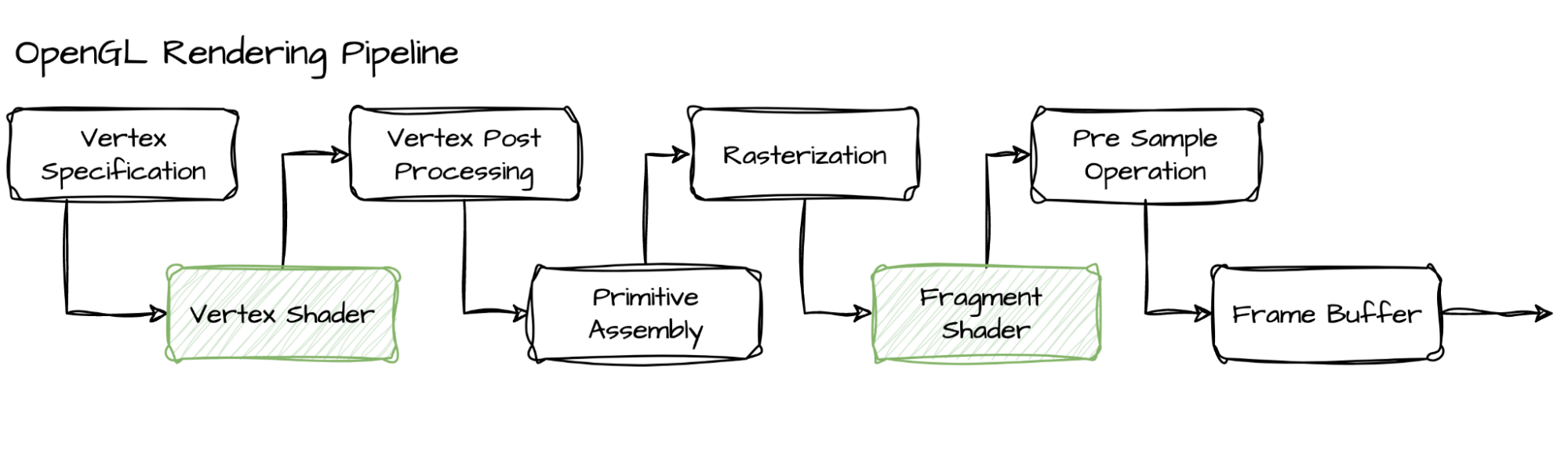
An example of OpenGL Pipeline
At this stage, it is enough to understand that a shader is a separate program, which we can write as plain text in a variable. Then, it can be compiled using RuntimeShader. After that, we will have an object that we can pass to the graphicLayers of a Compose element. We will use a regular Box for experiments. Thus, our Box will display the code written in the shader.
val runtimeShader = """ |
Shader program code
val shader = remember { RuntimeShader(runtimeShader) } |
Android code
This is the bare minimum required to run an ALSL shader in a Composable view. Let's immediately focus on two extremely important things here:
Even in the simplest shader, like ours, we need a parameter of type shader, which in this example is called image. It receives the contents of the RenderNode, and we will use this parameter in the future as it allows us to get information about the image under the element, which is necessary for effects interacting with the background, such as blurring or a glass effect. Just remember that this is a necessary minimum for the shader. Even though we do not use this variable, we still have to create it.
Despite the fact that our shader does not use any additional information and just outputs black color with half transparency, we need to set some color as a background for the Box, otherwise, it will not be displayed, and consequently, our shader will not be visible. In fact, instead of a background, we could have simply placed another element inside the box, it would still not be visible, because we ignore everything that should have been rendered since we ignore the image parameter. Just know that if you do not specify a color and do not put anything inside the box, due to the optimization of the Compose engine, it will not render this box at all. Therefore, let this line not confuse you, you can pass any color value and see that it does not affect the result.
Well, if everything is done correctly, upon launching the program, we will finally see our first shader.
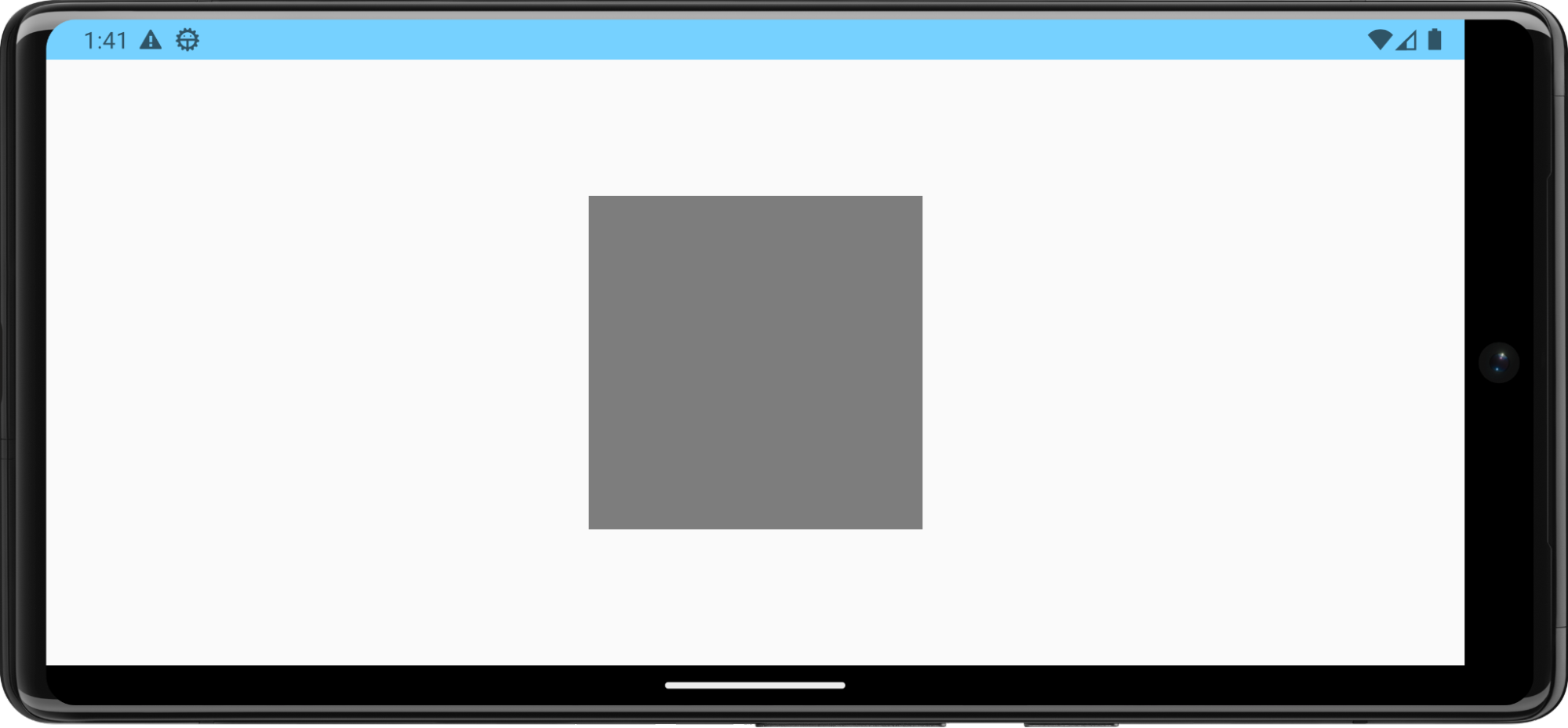
Note that if you forget to set clipToBounds, not only the box but the entire screen will turn gray. Again, this is because we ignore any parameters of the box, including its dimensions. We return a constant color for every pixel, and the canvas of the entire application is passed to the shader. Therefore, without this parameter, our shader will affect the entire screen |
For further experiments, I generated an image for the background. This will make the shader more visible. So, just keep in mind that the image in the following screenshots is simply a raster background. You can find it on my GitHub, the link is at the end of the book.
Let's now talk a bit about what happens in the shader code itself. So far, not much is happening, and this is a perfect moment to understand the basics. Essentially, we have one method that takes pixel coordinates and returns a color in the RGBA format, where each component can vary from zero to one. Zero means no presence, and one represents maximum intensity. Thus, the color red would look like half4(1.0, 0.0, 0.0, 1.0); Here, we have passed one for red (the first parameter) and one for alpha (the last parameter)
In general, simplifying greatly, think of the shader in this way: you receive a pixel coordinate, and you must answer the question—what color to return at that position. You may need additional parameters to answer this question, such as time, canvas dimensions, colors to apply, possibly an entire texture, and so on. But the essence remains the same—you have a pixel coordinate, and you decide what color that pixel will be
Currently, we are returning a constant color for all pixels, completely disregarding the coordinates. Let's try to take the coordinates into account. We will modify our shader so that the red channel depends on the pixel's horizontal position, and the green channel depends on the vertical position:
uniform shader image; | |
Shader program code | result |
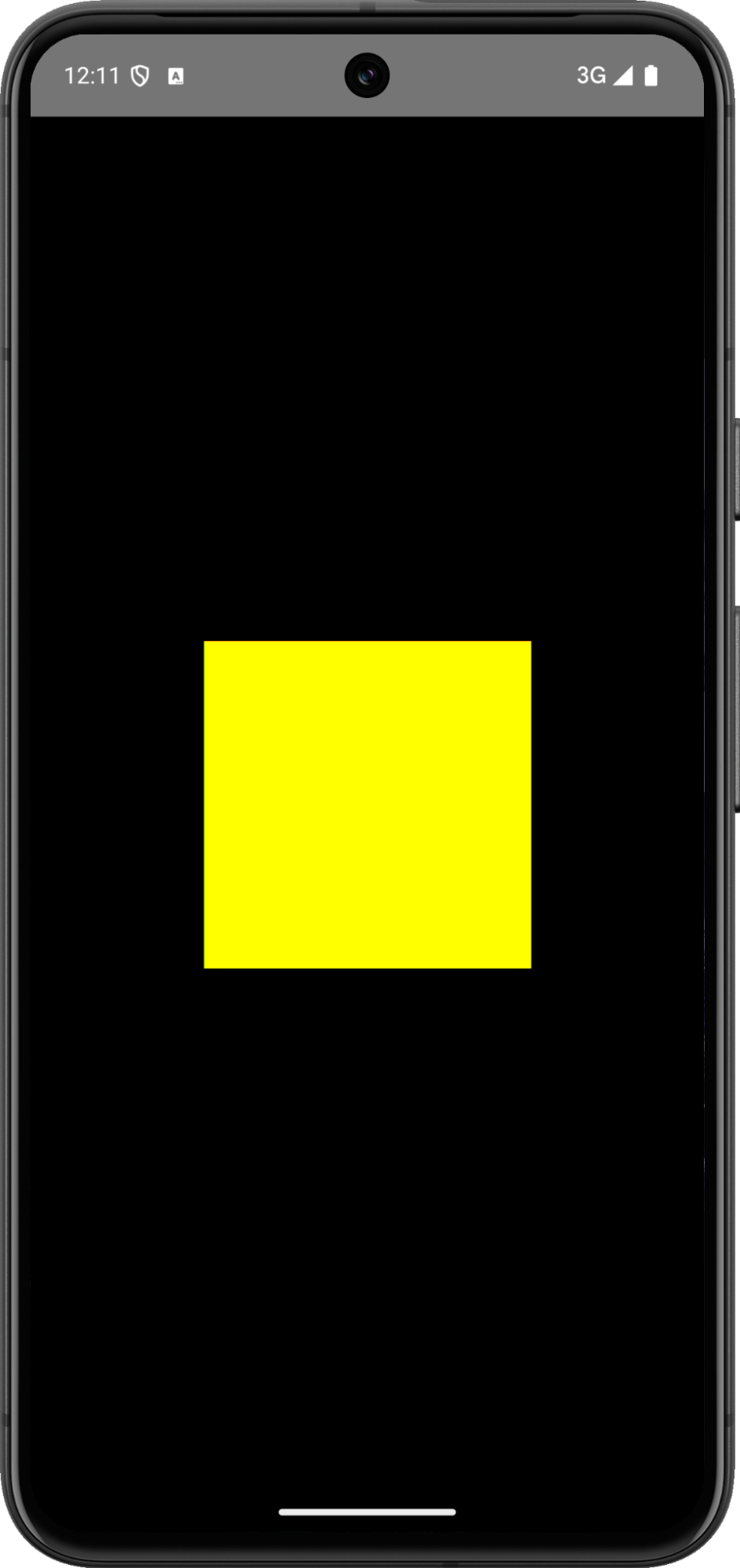
So now, our box has turned yellow. Not exactly what we might have expected. But really, what is yellow? It is a combination of red and green. Remember that the returned color should change from zero to one? Anything above one can also occur, but it appears as one because the color has already reached its maximum brightness. And the coordinates we receive are equal to the pixel coordinates, i.e., they change from zero to the size of the box. In other words, if our container size is 200 by 200 pixels, then we receive coordinates from zero to 199. To make everything work correctly, it is necessary to normalize the size of the canvas. In other words, map origin coordinates to new ones that would change from zero to one, where zero corresponds to zero in fragCoord, and one corresponds to the maximum (199 in the case if the container is 200 pixels in size).
To achieve this, it's necessary to know the dimensions of the container. Now, we'll see how additional parameters can be passed into the shader. First, we'll modify the shader code itself. Let's add a variable for the canvas dimensions: float2 resolution. And now we will obtain normalized coordinates, a variable historically named uv. Hence, we'll name the normalized coordinates the same. Altogether, our shader will now look approximately as follows:
uniform shader image; |
Shader program code
All that's left is to assign a value to resolution from our Compose code. We can determine the exact dimensions of the Box in the onSizeChanged modifier callback. That's where we will pass the data. It looks like this (remember, we are writing directly to the shader variable, so it's important that the names match):
Box(modifier = Modifier |
Android code
If everything is done correctly, the result should be as follows:
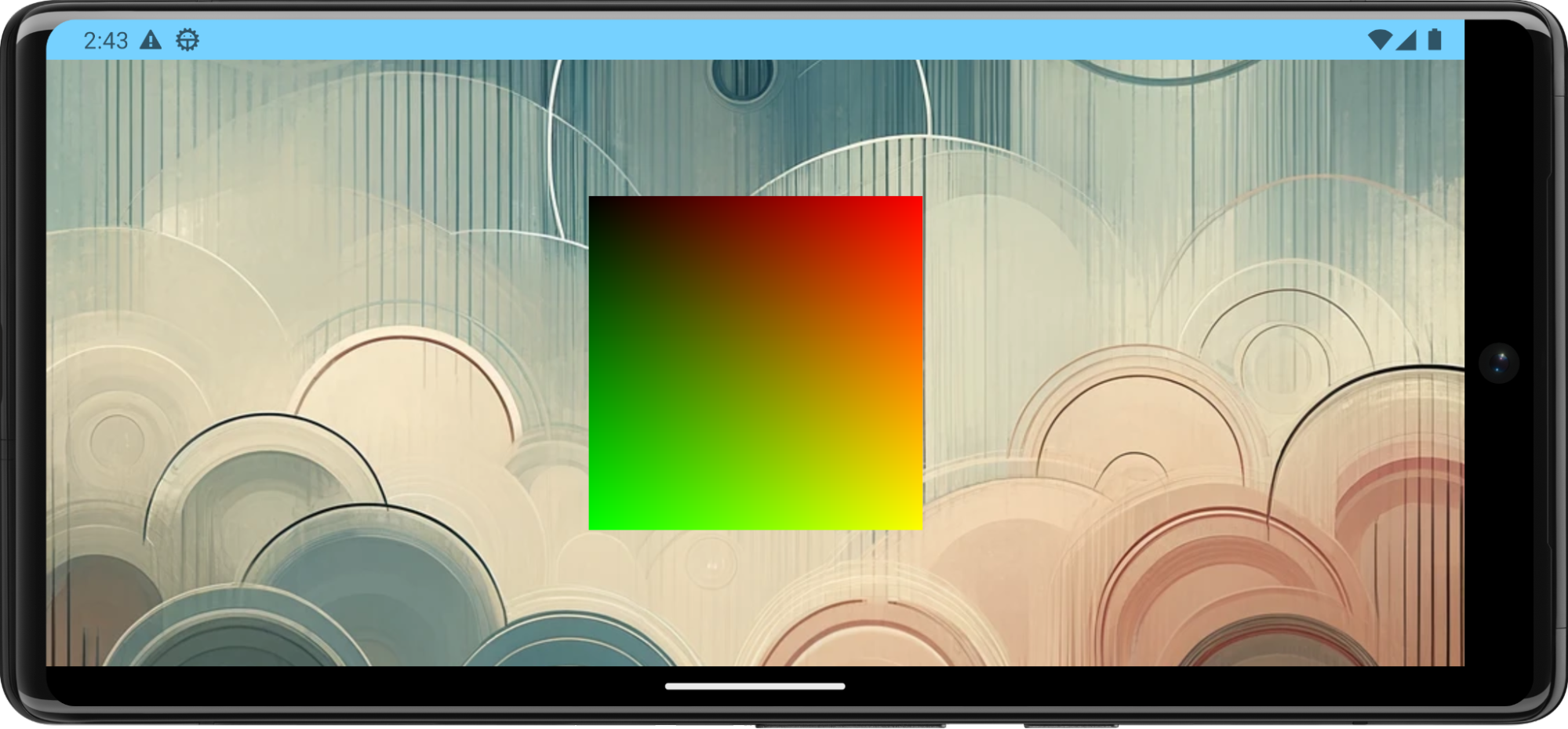
Here, you can see two clear gradients: the red channel changes horizontally, while the green channel changes vertically. At the end, diagonally in the bottom right corner, you can see yellow as a result of the merging of these two components. At this stage, I recommend experimenting with what we already have. Try altering the blue channel or the alpha. Try to make the changes not from zero to one, but the opposite, so that yellow appears in the top left corner. In short, let your imagination run wild and play around with it.
Section 02: Step function
Many like to describe shader programming as "painting with mathematics'' – and this is indeed a very accurate description of what happens. Instead of the familiar tools we use in traditional painting, like lineTo, moveTo, addRect, etc., we only have pixel coordinates (and possibly some other parameters) at our disposal, and we must somehow compute what we want to draw. We don’t move a brush; we calculate the color with formulas. Initially, this can feel very unusual and sometimes even dauntingly complex. But with time, you get used to it, and later, you come to realize just how powerful a tool you have.
And since we will be painting with formulas here, I am convinced that it is extremely important to understand their meaning.
Let’s start with probably the most common function. It is called step.
genType step(genType edge, genType x);
x - Specify the value to be used to generate the step function. Description step generates a step function by comparing x to edge. For element i of the return value, 0.0 is returned if x[i] < edge[i], and 1.0 is returned otherwise. source: https://registry.khronos.org/OpenGL-Refpages/gl4/html/step.xhtml |
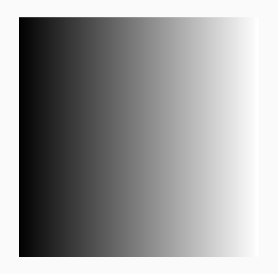
We already drew a gradient in the previous section. Now let's modify it so that only the horizontal part changes. We'll apply this to all three colors. This way, we'll create a horizontal black-and-white gradient.
half4 main(float2 fragCoord) { float2 uv = fragCoord / resolution; } | |
Shader program code | result |
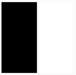
And now let’s say we want instead of a gradient to get just an edge. So, for some level it should be black and then immediately turn to white. That is where step function comes into play.
half4 main(float2 fragCoord) { float2 uv = fragCoord / resolution; float value = step(0.5, uv.x); float3 color = float3(value, value, value);
return half4(color, 1.0); } | |
Shader program code | result |
Now let’s try to draw something more complex. For instance, draw a line. Currently our coordinates are in a range from 0 to 1. We can move it on a half to the right. It will make the origin be right in the middle of the canvas. It has a lot of benefits, and now we will use one of them: since the horizontal axis after movement changes from -0.5 to 0.5, we can use absolute values to get two edges for the price of one!
half4 main(float2 fragCoord) { | |
Shader program code | result |
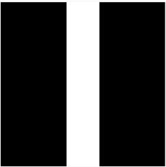
Similarly we can add a horizontal line using the vertical component of the uv. Adding altogether gives us a “plus” symbol:
half4 main(float2 fragCoord) { | |
Shader program code | result |
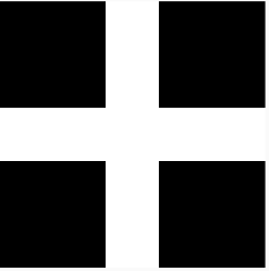
Notice how here we used what's called vector swizzling, on the following line: float3 color = float3(horizontal+vertical); In other words, in GLSL (and other shader programming languages), mathematical operations are so common that vector manipulation is highly advanced. I’ve created float3 from a single number, which would look like this: float3 a = float3(0.0); and it would be equivalent to float3 a = float3(0.0, 0.0, 0.0); And also take a look on: return float4(color, 1.0); Instead of passing directly all four values, I’ve just got a three dimensional vector (float3) and then added only one additional param for the alpha and it gives me a float4 vector. |
Let's think about how we might draw a circle in a shader? For this, we need to recall what a circle consists of. Generally, it has a radius and a center. Let's, for simplicity, place the center at the origin (Already the second benefit of moving uv coords to be centered at zero point). That leaves only the radius. It turns out, if a point is closer to the center than the radius, it's inside the circle; if further, it's outside.
Let's recall the formula for a circle: . In our case, the coordinates are represented by uv, so we can express the radius of the circle as . Now, we can compare the current point to this formula to determine whether it falls within the circle. Accordingly, we can assign a value of 1 if it is inside the circle and 0 if it is outside using step function


half4 main(float2 fragCoord) { step(sqrt(uv.x * uv.x + uv.y * uv.y), radius); | |
Shader program code | result |
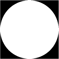
Let's now take a closer look at the part of the code that defines the circle. Essentially, this is the Pythagorean theorem, where the distance acts as the hypotenuse. If we were to draw a line segment that starts at the origin and ends at the coordinates of our uv vector, we would get a right triangle with legs equal to the values of uv.x and uv.y. Therefore, the length of uv will be exactly

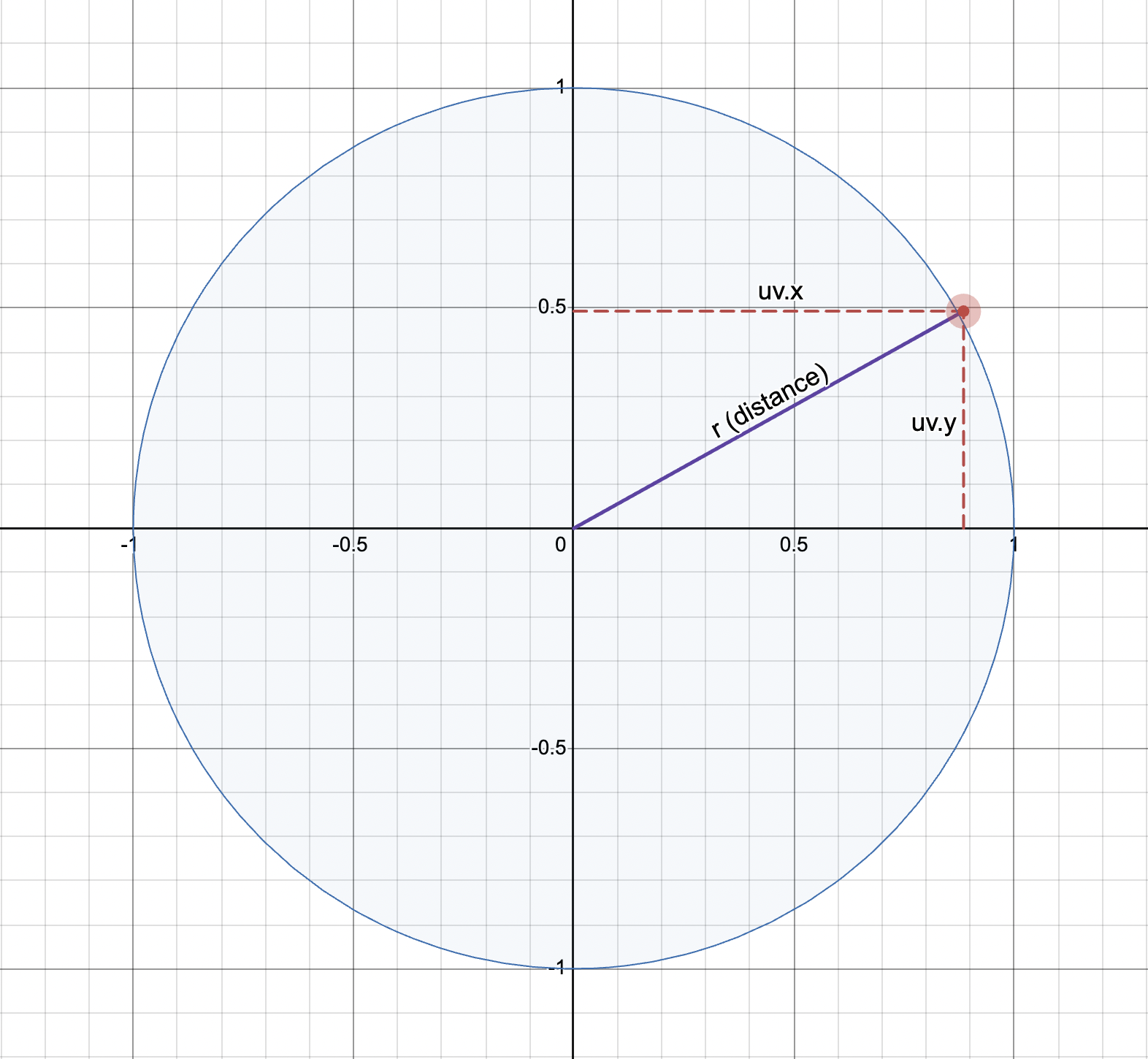
Red point represents a random UV coordinate. Circle is just an illustration that shows that distance is actually a radius.
The good news is that GLSL has a built-in function for this operation. It's called length and it takes a vector as input. The result will be its length, or the distance from the origin to the coordinates of the vector.
sqrt(uv.x * uv.x + uv.y * uv.y); |
Name length — calculate the length of a vector float length(genType x); Description length returns the length of the vector, i.e source: https://registry.khronos.org/OpenGL-Refpages/gl4/html/length.xhtml |
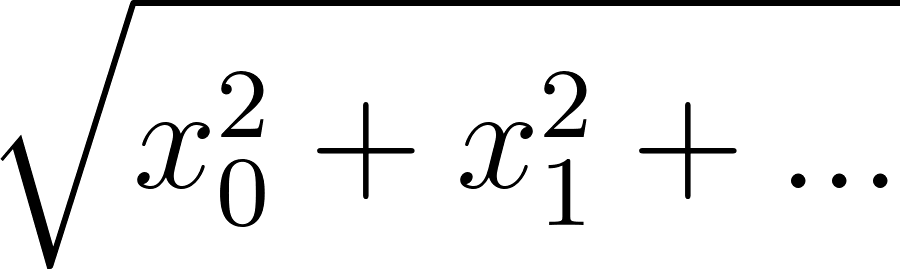
Now we can extract the variable for the circle and name it appropriately. Let's also create a variable for the color. We will obtain the final color by multiplying the circle's value by a predetermined color. This is a very common practice in shaders, so get used to this approach. We have some formula that simply returns a value for a given coordinate, and then, we multiply this value by a specified color to thus obtain the final image. Moreover, we can now also apply this same value separately to the alpha channel, so our shader won’t be black at the corners. Bringing together everything we just discussed, we get the final code for our circle:
uniform shader image; | |
Shader program code | result |
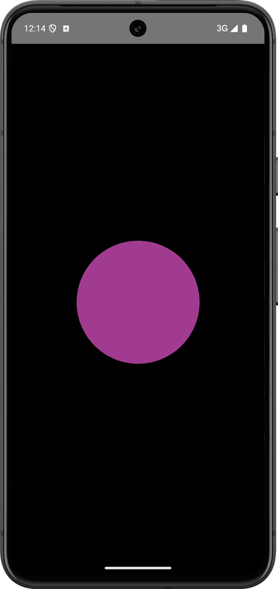
The step function takes an edge and the value of the function, so it's more accurate to use it in reverse: step(radius, length(uv)). However, in such a case, there will be an inversion of values, with zero outside the circle and one inside. Consequently, we need to subtract one, and the final code would look like this: float circle = 1 - step(radius, length(uv)); On the other hand, the initial writing is also correct, so it more depends on personal preference. |
Section 03: Smoothstep
If we plot the graph of the step function, we'll notice that it is discontinuous and has a break at the point where its value transitions from zero to one.
In that example, t = 0.1 and we see how step fun changes there its value | In that example, t1 = 0.1 and t2 = 1.3. We see how smoothstep fun changes there its value |
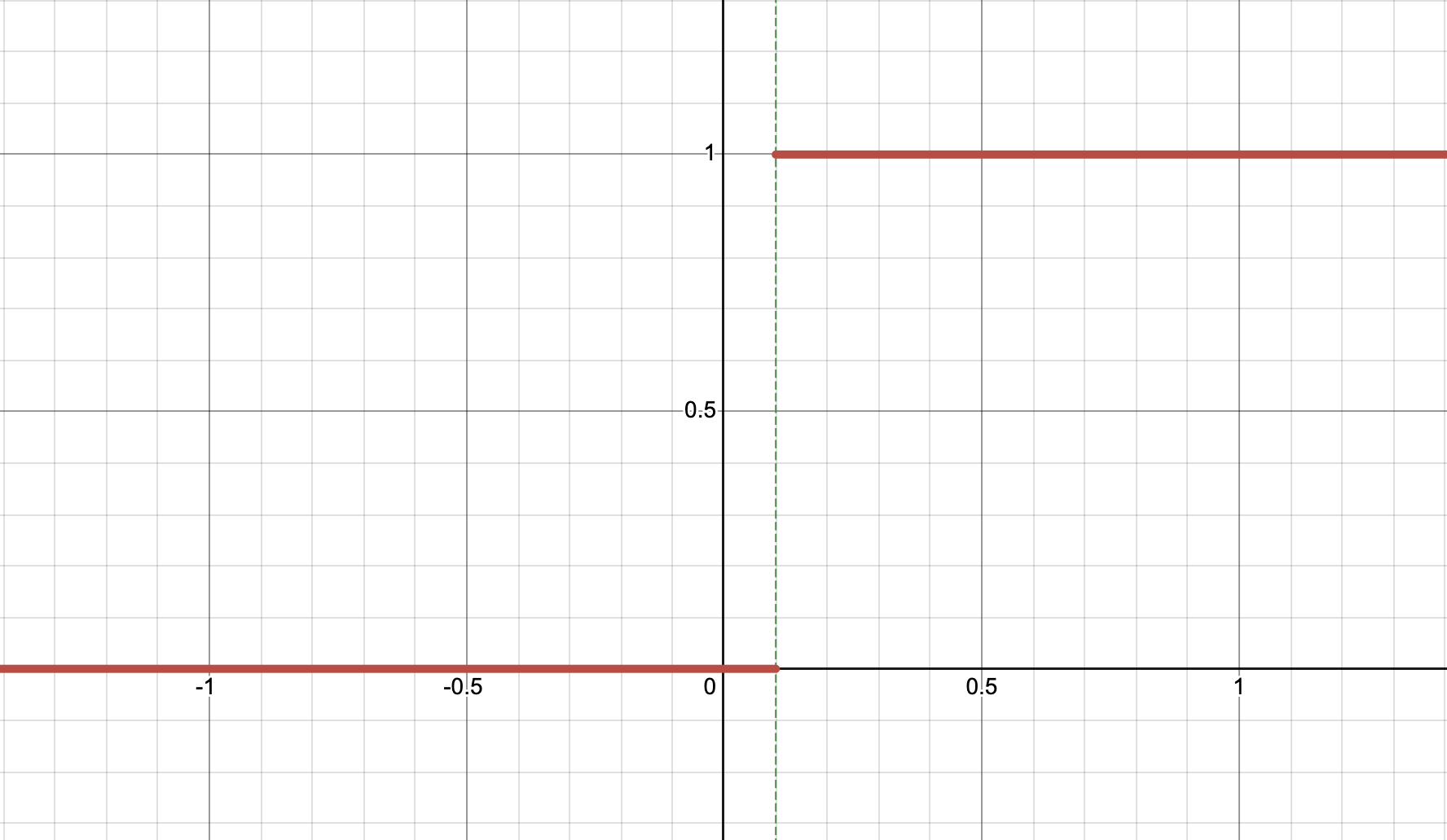
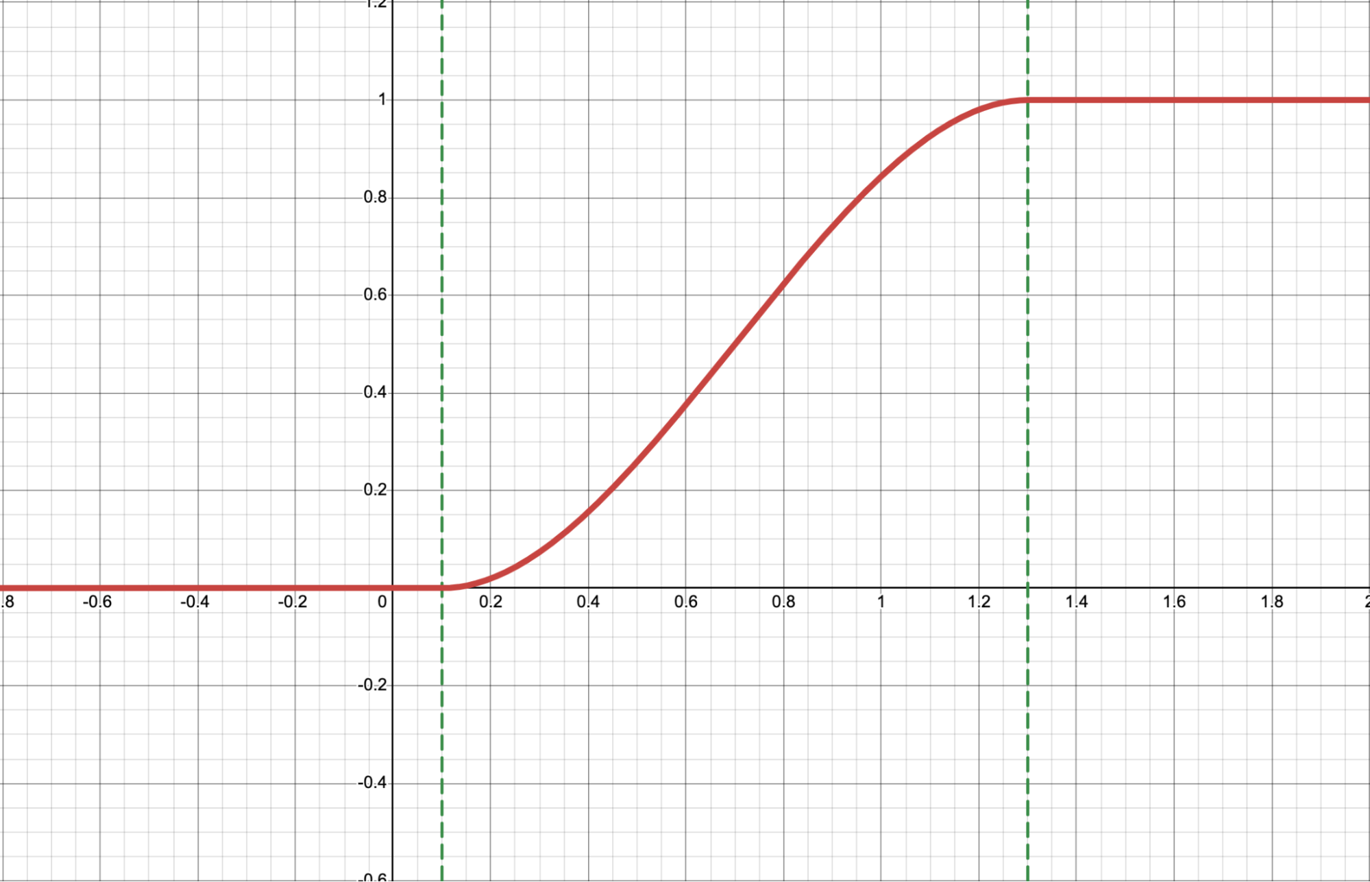
As a result, we end up with a very rough edge on the circle. It is literally jagged, since one pixel had maximum color intensity, while the adjacent one had no color at all. We would like to have a smoother transition. If depicted on a graph, we would like to see a smooth interpolation from zero to one, as shown below
This is exactly how smoothstep functions in GLSL. This method takes three values: the left edge, the right edge, and the current value for interpolation. It returns a number equal to 0 if it is less than the left value, 1 if it is greater than the right value, and an interpolated number if the value is within the range. Understanding this, we can change our shader code from using step to smoothstep:
float circle = smoothstep(radius, radius-0.03, length(uv)); |
Shader program code
Name smoothstep — perform Hermite interpolation between two values genType smoothstep(float edge0, float edge1, genType x); edge0 - Specifies the value of the lower edge of the Hermite function. edge1 - Specifies the value of the upper edge of the Hermite function. x - Specifies the source value for interpolation. Description smoothstep performs smooth Hermite interpolation between 0 and 1 when edge0 < x < edge1. This is useful in cases where a threshold function with a smooth transition is desired. smoothstep is equivalent to: genType t; source: https://registry.khronos.org/OpenGL-Refpages/gl4/html/smoothstep.xhtml |
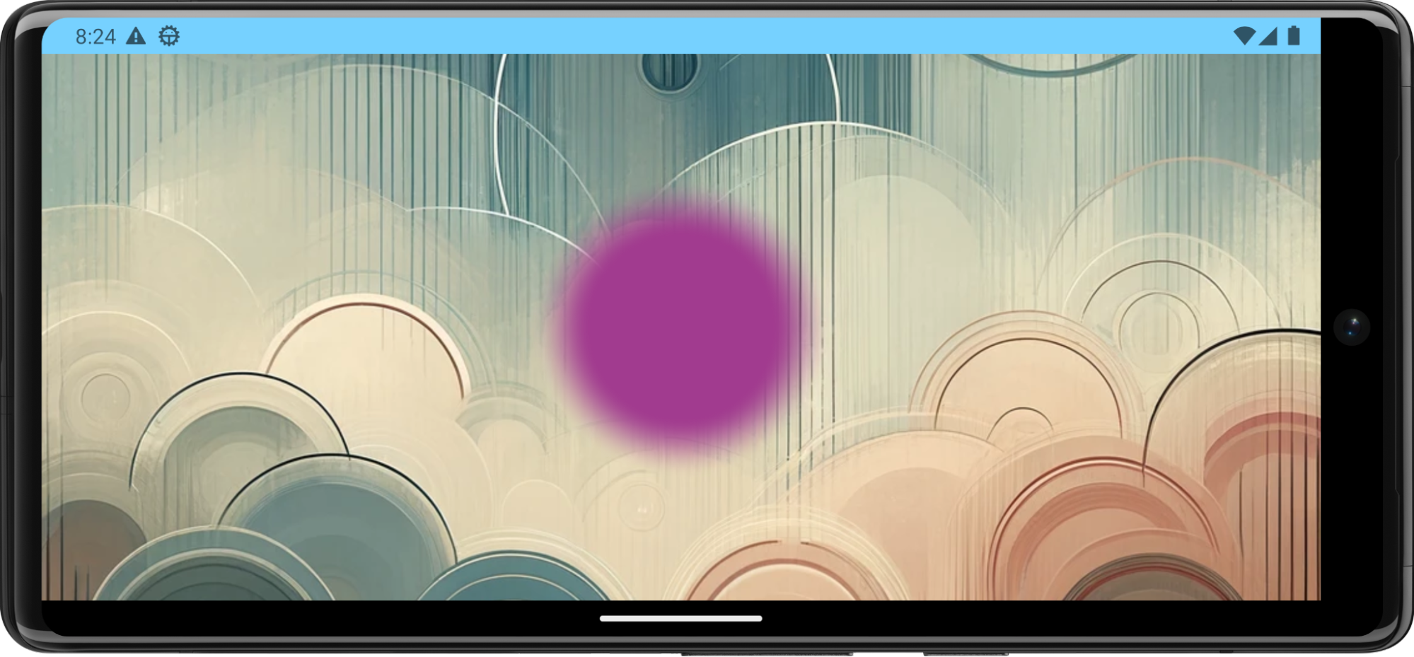
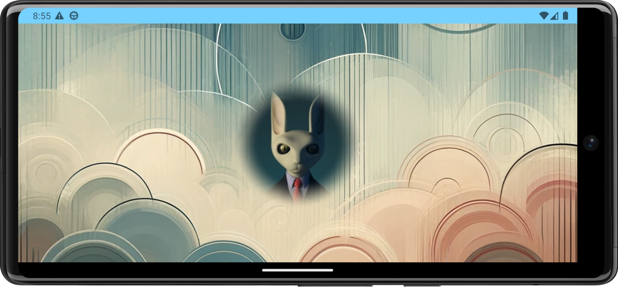
Right now, we are defining the color in the shader based solely on the pixel's position. We are not considering the image that is inside the Box, so if we add something to the Box now, we'll notice that it does not display. Let's fix this. Do you remember that we bind the shader to a variable called image? With it, you can obtain the color of the current pixel that would exist without our shader. This can be done using the eval method. Then, you can combine this with the circle to create a beautiful, soft gradient transition from the image to the background.
At this stage, I will again provide the full code of the shader and the Compose component (the avatar is simply loaded from resources as a raster image):
val runtimeShader = """ |
Shader program code
VerySimpleShaderTheme { |
Android code
Note that our shader draws a circle only if the container has square dimensions. If it is a rectangle, our circle will be deformed. To account for this compensation, we need to adjust the uv coordinates. This can be done as follows: uv.x *= resolution.x / resolution.y; |
Section 04: Signed Distance Function
We've already learned how to draw a circle. Now, using the techniques we know, let's think about how to draw a ring? The answer is surprisingly trivial: draw a second, smaller circle and subtract it from the first one.
float4 main(float2 fragCoord) { | |
Shader program code | result |
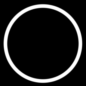
This works great. But it looks a bit complicated. At that point it is a good moment to dive into SDF (Signed Distance Function). An SDF represents a way to describe a shape or an object in a spatial grid by assigning each point in that grid a value. This value indicates the shortest distance from that point to the surface of the shape. The "signed" part of the name comes from how these distances are recorded: distances outside the shape are usually given as positive values, while distances inside the shape are negative.
You can find a lot of SDFs for different sorts of shapes. Here is a link to a great collection of that: https://iquilezles.org/articles/distfunctions2d. And if you take a look there, the SDF for circle would be the following:
float sdCircle(vec2 p, float r) |
Let’s try to visualize it. For that let’s remove clipToBounds on our Box component, so we can see our shader even out of Box bounds and apply the following shader to it:
uniform shader image; float sdCircle(vec2 p, float r) { float4 main(float2 fragCoord) { float outerDist = clamp(dist, 0., 1.); float3 col = circle * float3(outerDist, innerDist, 0.); col = mix(col, float3(1.0), smoothstep(0.01, 0.0, abs(dist))); | |
Shader program code | result |
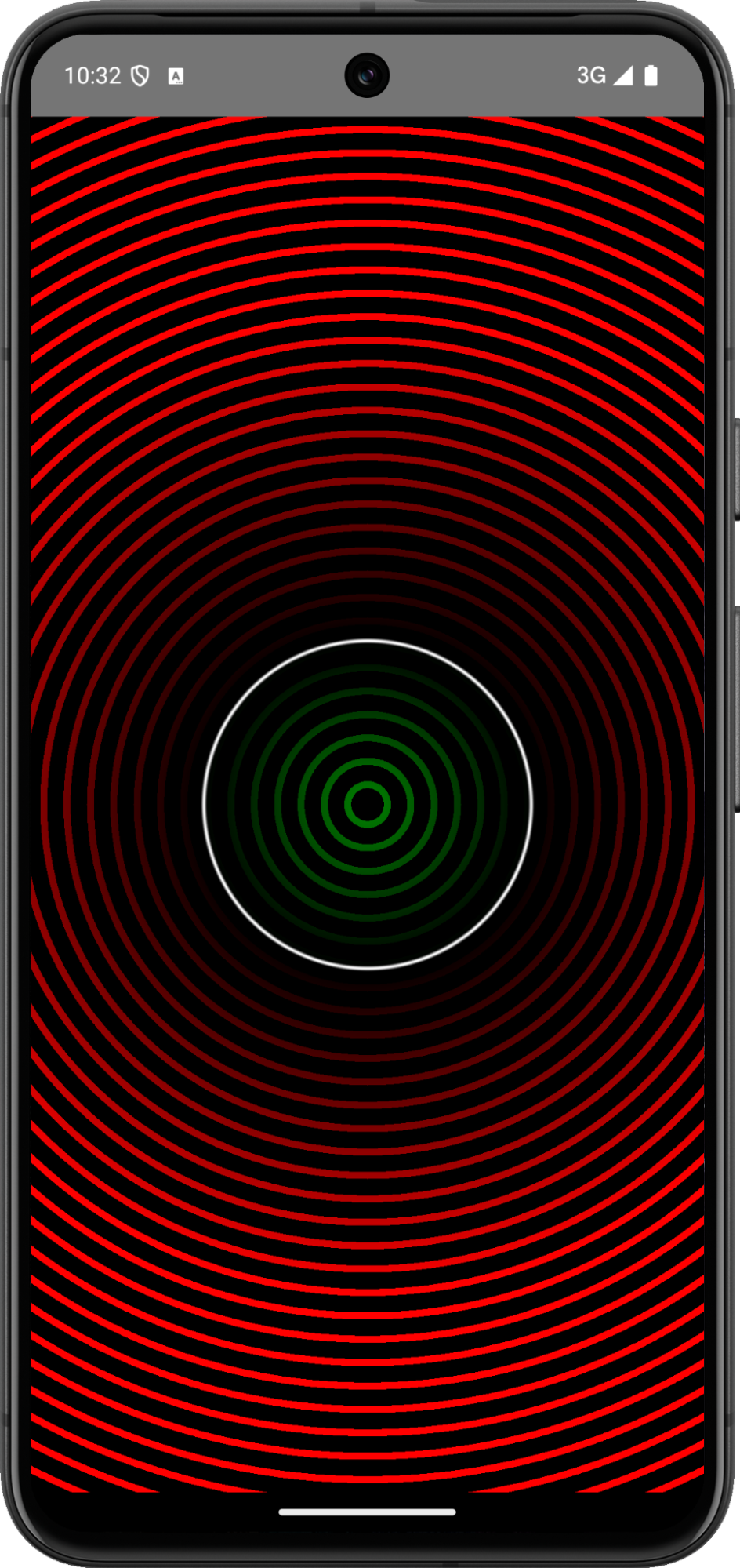
In all following code snippets I will mark methods with blue color, if these methods already were described in this book before. So I wouldn’t repeat myself and will try to keep snippets compact and clear. If you will see such methods, you will know that they are not built-in in GLSL and have to be written by yourself before the main method. |
In this shader, we introduced several new methods. Let's take a closer look at how they work. First, let's focus on the fract method. It returns the fractional part of a number. For example, if you input 1.33, you get 0.33, if you input 4.5, you get 0.5, and so on. We will often use it to divide the canvas into smaller sectors. Remember that our UV varies from -0.5 to 0.5. If you multiply UV by 2 and call fract, you will get 4 squares, ranging from 0 to 1. Below, I've provided an example with a visualization of this method, using a gradient for clarity
float4 main(float2 fragCoord) { float2 uv = fragCoord / resolution - 0.5; uv = fract(uv*2.0); } | |
Shader program code | result |
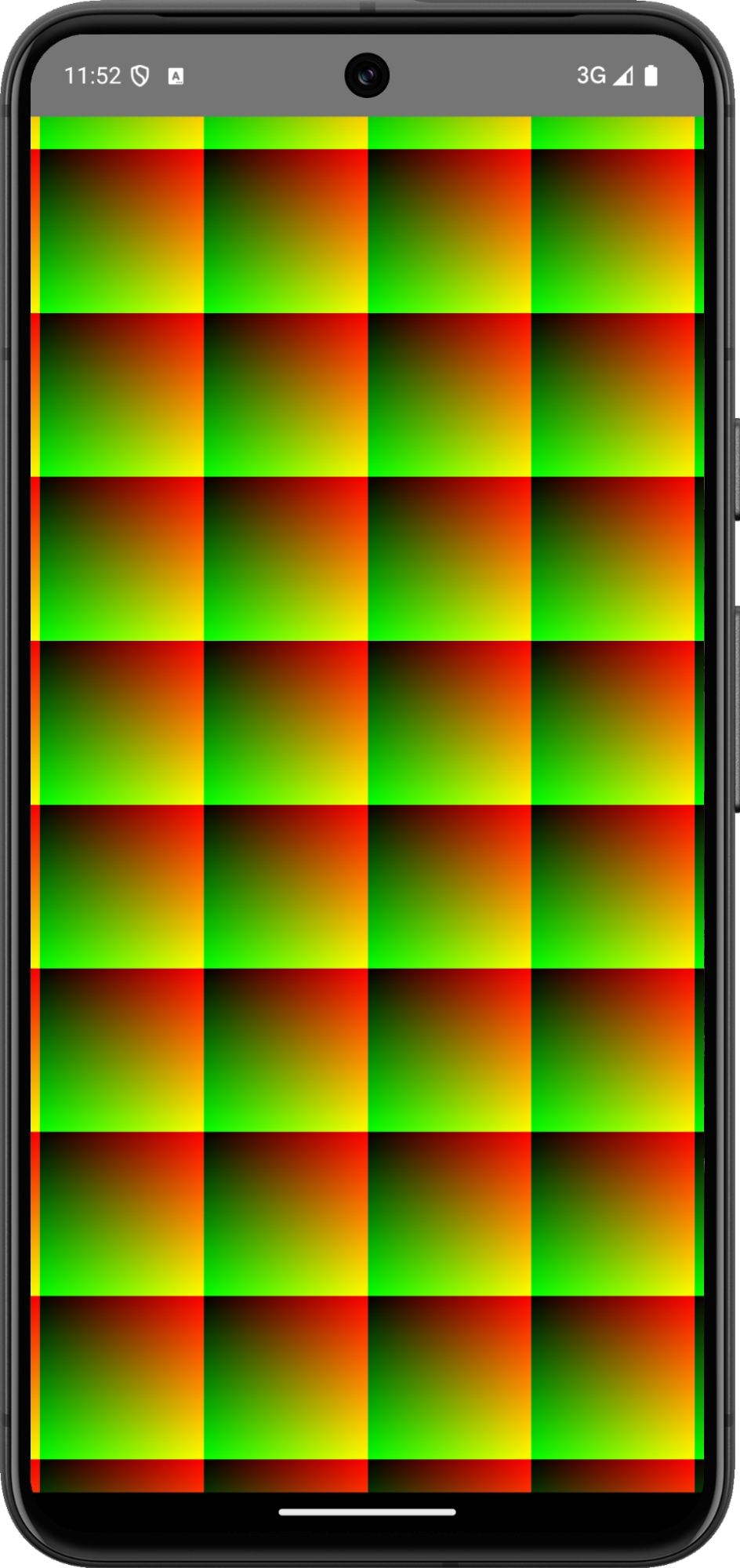
Name fract — compute the fractional part of the argument genType fract(genType x); x - Specify the value to evaluate. Description fract returns the fractional part of x. This is calculated as x - floor(x) source: https://registry.khronos.org/OpenGL-Refpages/gl4/html/fract.xhtml |
So, we multiplied the coordinates by 14 and took the fractional part, thereby obtaining many small sections from zero to one. Next, we called step for the obtained SDF value of the circle and some predefined value (0.7 in our case), thus creating many circles. Pay close attention to this line, it is very important to understand this principle and why it works this way. In the future, we will often resort to a similar method. Essentially, in any effect where there are many small, similar, or even identical elements, we will use fract.
Note that we do not change our dist variable itself, we just use it to get many similar distances on a smaller area of the canvas. So further we will use the original dist value for calculations, and it has nothing in common with that fract value.
Next we are extracting two new values from our dist:
float outerDist = clamp(dist, 0., 1.);
float innerDist = abs(clamp(dist, -1., 0.));
As you remember, SDF stands for signed distance, so it will be greater than zero outside our shape and less than zero inside it. To use it separately for coloring our rings, I’m using a clamp method from the GLSL.
Name clamp — constrain a value to lie between two further values genType clamp(genType x, genType minVal, genType maxVal); x - Specify the value to constrain minVal - Specify the lower end of the range into which to constrain x maxVal - Specify the upper end of the range into which to constrain x Description clamp returns the value of x constrained to the range minVal to maxVal. The returned value is computed as min(max(x, minVal), maxVal). source: https://registry.khronos.org/OpenGL-Refpages/gl4/html/clamp.xhtml |
Thus, we ended up with two variables that increase from zero, but one is only for positive SDF values, and the other for negative ones. Now, by using one value for the red channel and the other for the green, we will achieve different colors for the outer and inner rings.
Overall, we could have finished at this point, using this value as the final color. However, I decided to add a white ring, marking the spot where the SDF equals zero. This was done using a technique already familiar to us, with the help of smoothstep. Since the SDF equals zero at the boundary of the shape, by taking the absolute value and setting the edges from 0.01 to 0.0, we get a ring that spreads out in both directions from the edge, but with a width of 0.01.
smoothstep(0.01, 0.0, abs(dist))
But our code also includes the mix method. This method allows for linear interpolation between two values. Mix is used when it's necessary to combine two different shapes in one shader. We specify both shapes and a value from zero to one, describing which of them needs to be displayed at a particular spot. At a value of 0, the first shape will be displayed, at 1, the second, and at values between 0 and 1, the shapes will blend in the specified proportion
Name mix — linearly interpolate between two values genType mix(genType x, genType y, genType a); x - Specify the start of the range in which to interpolate. y - Specify the end of the range in which to interpolate. a - Specify the value to use to interpolate between x and y. Description mix performs a linear interpolation between x and y using a to weight between them. The return value is computed as x×(1−a)+y×a source: https://registry.khronos.org/OpenGL-Refpages/gl4/html/mix.xhtml |
That's it! We've covered the visualization of the SDF method. As an example, we could try some other shape instead of a circle. On the website with SDF functions that I mentioned, there are links to ready-made visualizations using GLSL. And they too effectively demonstrate the essence of SDF. However, first of all, it's always more interesting to do something on your own, and secondly, their method seems overly complicated and difficult to understand for beginners. Moreover, by visualizing in your own way, you better understand the method itself. I hope I've explained my implementation in detail. If anything remains unclear, I strongly recommend rereading and delving deeper. We will continue to frequently use all the described techniques, but I won't stop to explain them again in order to keep the description concise.
EquilateralTriangle SDF | Pentagon SDF | Hexagram SDF |
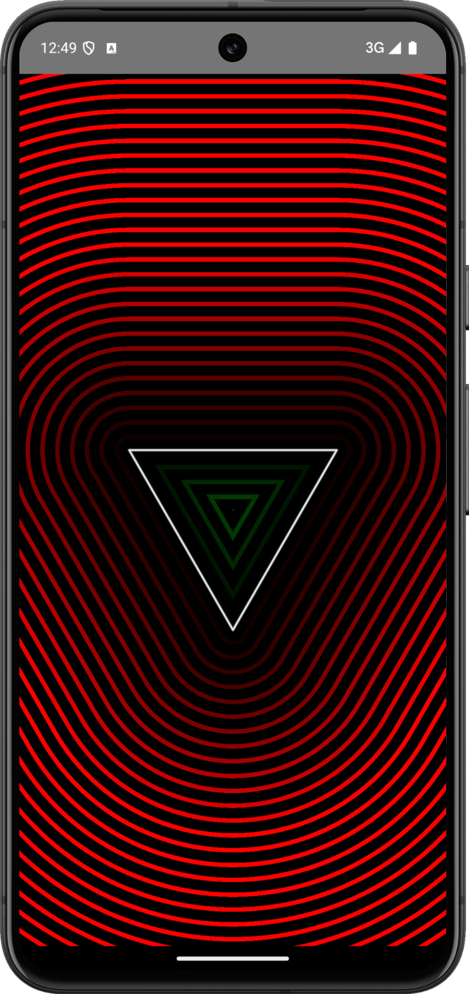
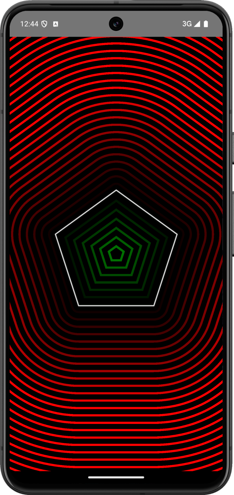
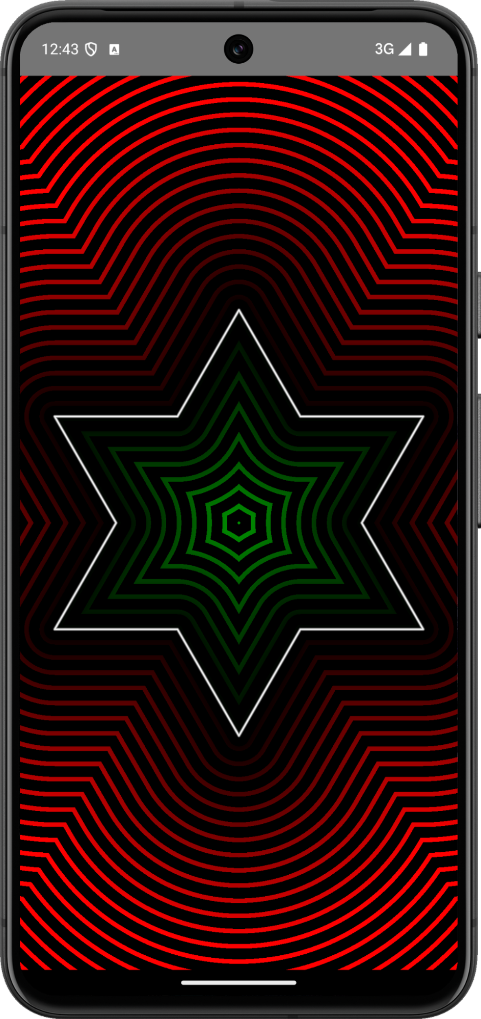
In some SDF shapes from the link above they are using the dot2 method. It is not a standard GLSL method, if you want to be able to compile shapes that are using that method, add before the shape method the following: float dot2(in vec2 v ) { return dot(v,v); } |
Using SDF (Signed Distance Functions) is convenient for creating glow effects on various UI components. We will talk more about different types of glows later in this book, but I am already eager to show you something really interesting and exciting. So, before we move on, let’s try applying everything we have learned about shaders so far and create a glow effect for a standard button. We'll start by writing an SDF method to obtain a rectangle with rounded corners. It can be done as follows
float sdRoundedBox( in vec2 p, in vec2 b, in vec4 r ) | |
Shader program code | result |
Let's create a composable function that will internally create a button and apply our shader to it:
@Composable
fun GlowButton(
modifier: Modifier = Modifier,
text: String
) {
val shader by remember { mutableStateOf(RuntimeShader(shader)) }
OutlinedButton(
modifier = modifier
.onSizeChanged { size ->
shader.setFloatUniform("resolution",
size.width.toFloat(),
size.height.toFloat()
)
}
.graphicsLayer {
this.renderEffect = RenderEffect
.createRuntimeShaderEffect(shader, "image")
.asComposeRenderEffect()
},
onClick = { }) {
Text(text)
}
}
And the usage of that button might looks something like that:
class MainActivity() : ComponentActivity() {
override fun onCreate(savedInstanceState: Bundle?) {
super.onCreate(savedInstanceState)
setContent {
RuntimeShadersTheme {
Box(
modifier = Modifier
.background(MaterialTheme.colorScheme.background)
.fillMaxSize(),
contentAlignment = Alignment.Center
) {
GlowButton(text = "Hello, glow!")
}
}
}
}
}
Now let's add the usual routine code for coordinates and include the use of SDFRoundedBox.
float4 main(float2 fragCoord) { // setup a rounded rect shape: vec2 d = vec2(0.5 * ratio, 0.4); //assign shape to a color vec3 col = shape*vec3(1.0); // just white color for now | |
Shader program code | Result |
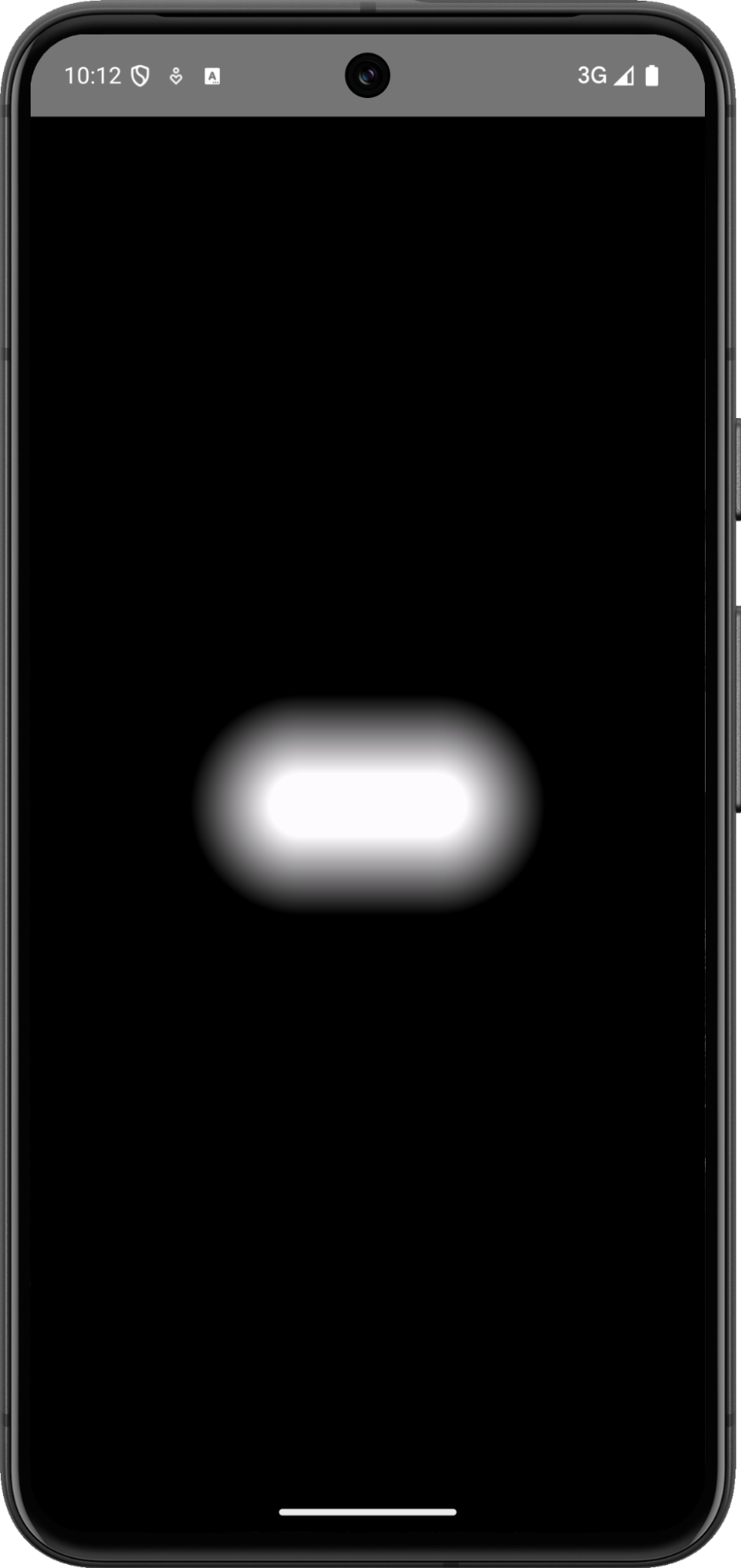
If everything is done correctly, the result should look something like the screenshot above. It's not too impressive yet, but we're close to turning this into something truly spectacular. I deliberately didn't give all the shader code at once because it's important for you to see this crucial stage. The thing is, by obtaining the shape using SDF (or any other method), we've achieved the most important part. Coloring it, playing with the gradient strength, and other adjustments will soon become second nature to you. This is exactly the point where you can start the relaxing process of transforming this indistinct blot into a beautiful glow. Let's think, what do we need for this? First, we must get the image of the button itself and cut the button out from our shader so it doesn't draw over it. We have already obtained the image from the system, which is done through the variable 'image' using the eval method. We will cut out using the alpha channel. Finally, we need to combine our calculations and the image of the button, which is done using the mix method
float4 main(float2 fragCoord) { float shape = clamp(sdRoundedBox(uv,d,r),0.,1.); vec3 col = mix(img.rgb, vec3(0.0), clamp(shape-img.a,0.,1.)); | |
Shader program code | Result |
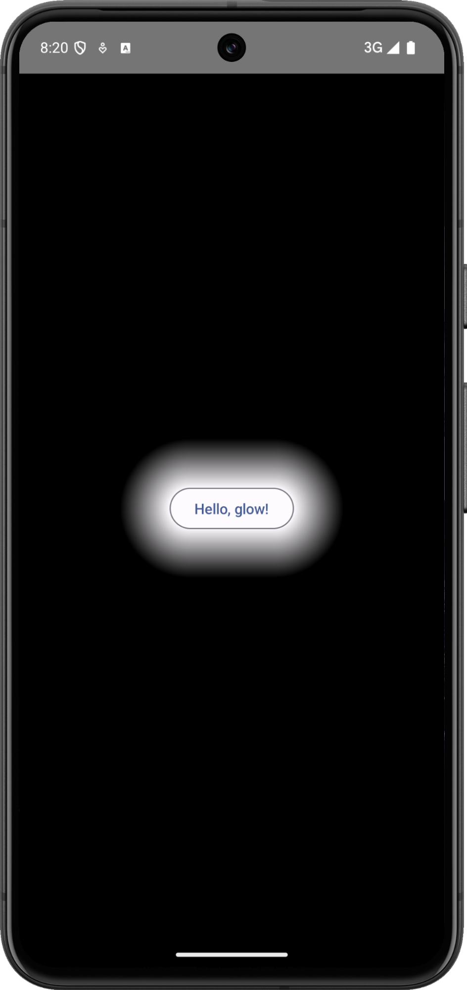
It's important to note that at this stage, the shader completely overwrites the background and everything on it, so the appearance of the application depends on the colors of the button. Therefore, it's crucial to choose a light theme on the phone, otherwise the image may not be visible at all, since the button colors will be white and our shader paints everything white, resulting in nothing being visible. So, turn on the light theme and use the standard theme to get the correct result at this stage |
We see that the background is black after applying the gradient. This happens because the SDF function returns the distance to the edge, and this distance increases the further from the edge you are. In our shader, we use a clamp between zero and one, i.e., beyond a certain distance, our shape always returns 1. The logic currently in use for blending the final color is this: mix(img.rgb, vec3(0.0), clamp(shape-img.a, 0., 1.)). This means that if the shape equals 1 and the button's alpha is zero, we will use the second value, i.e., vec3(0.0), so everything that is far enough from the button will have vec3(0.0) or, in other words, be black.
Let's make some adjustments. First, instead of using a predefined black color, let's pass the color from the Compose method. We'll call it baseColor. Next, we'll create a smooth gradient that will be intense near the edges and then gradually fade and approach zero: clamp(1./(25.*sdRoundedBox(uv,d,r)), 0., 1.). All that's left is to apply this to the final color, and as a result, our shader will look as follows:
float4 main(float2 fragCoord) { |
Since our main container has a Material Theme background color, we will pass as a baseColor a color from the Material Theme, that is used for onBackground:
@Composable fun GlowButton( modifier: Modifier = Modifier, text: String ) { val color = MaterialTheme.colorScheme.onBackground val shader by remember { mutableStateOf(RuntimeShader(shader).also { it.setFloatUniform("baseColor", color.red, color.green, color.blue) }) } … //rest of the app | |
Compose code | Result |
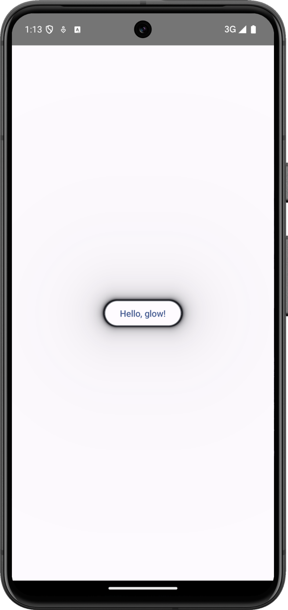
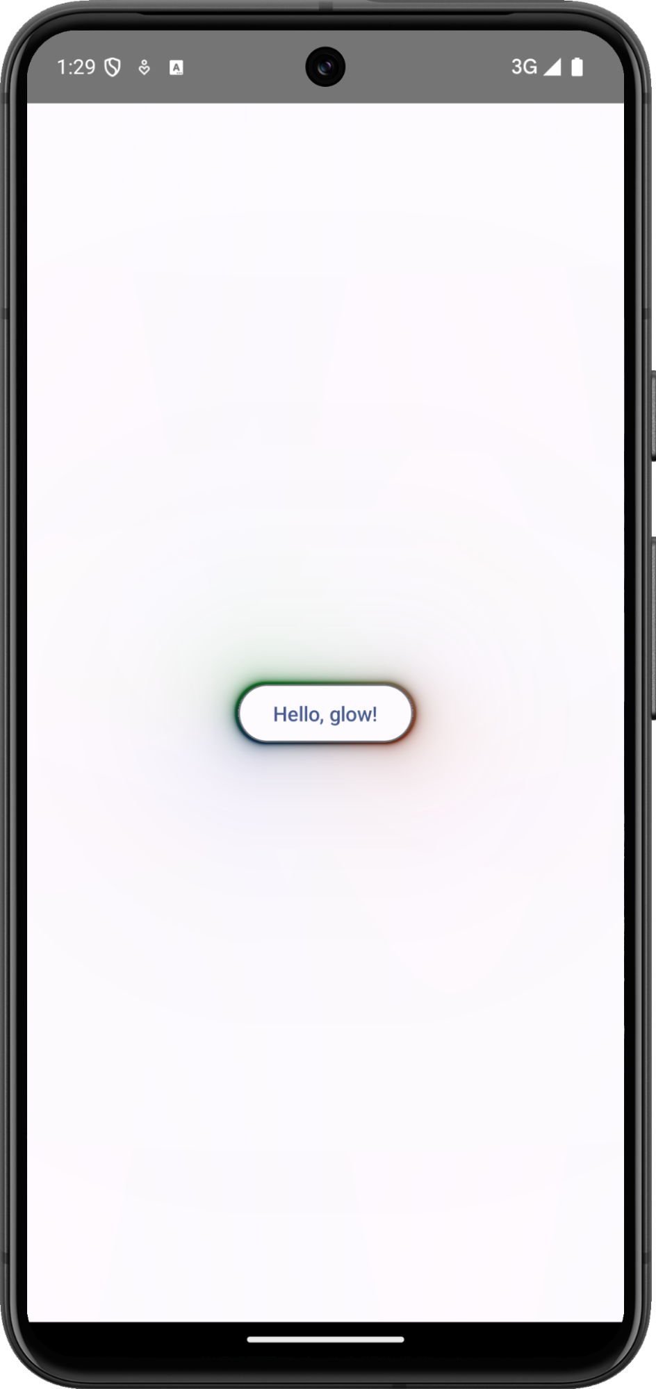
Additionally, instead of passing just one color, we can create a gradient and make it 'live' by using time. In fact, for various effects, we often need to use time, so now is a good moment to write a small helper method that will serve as a sort of stopwatch for us:
@Composable
fun provideTimeAsState(initialValue: Float = 0f): State<Float> {
val timeState = remember { mutableFloatStateOf(initialValue) }
LaunchedEffect(Unit) {
while (true) {
timeState.floatValue += 0.01f
delay(10)
}
}
return timeState
}
Now, to use it we can simply add another variable in our GlowButton fun:
val time by provideTimeAsState()
An important thing to note is that this variable needs to be passed to the shader in the graphicsLayer block, as it changes. If we pass it elsewhere, it will not affect our shader:
.graphicsLayer {
shader.setFloatUniform("time", time)
this.renderEffect = RenderEffect
.createRuntimeShaderEffect(shader, "image")
.asComposeRenderEffect()
}
Now, all that's left is to create a variable for time in the shader itself, as well as create a beautiful gradient and use it in conjunction with the base color. As a result, we will get our final outcome:
uniform shader image; + length(max(q,0.0)) - r.x; vec4 img = image.eval(fragCoord).rgba; vec3 col = mix(img.rgb, grad, shape); | |
Shader Program code | Result |
Section 05: Angle to the point
We've already become quite proficient with SDF methods for creating various shapes. Let's return to rings. I think the following shader will now raise no questions:
float4 main(float2 fragCoord) { abs(sdCircle(uv, r))); | |
Shader program code | result |
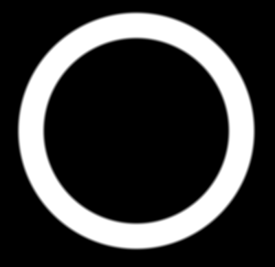
We're already able to increase the blur of edges, change the radius, and add gradient fill. Not few, but not too many tools in our arsenal either. In this section, I would like to talk about distorting the actual line of the ring. Suppose we want the ring to be not smooth, but wavy. Of course, we could look for the appropriate SDF function, but let's try to do this on our own. Usually, when we hear the term 'wavy line' the first thing that comes to mind is a sine wave. Take a look at its graph if it doesn't immediately come to mind:
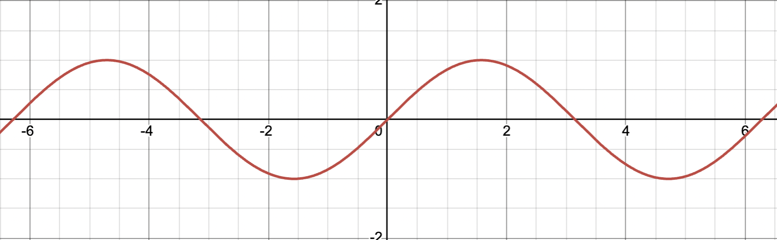
Imagine a ring as if it were a simple function, and r as its constant value on the x-axis. This makes the function's graph a straight, horizontal line. Essentially, we are seeing this line, but it's twisted into the shape of a ring. By knowing the angle at each point on the ring, we can adjust the radius accordingly. Think of using the angle as if it were the x-axis value.
Let's make this more concrete with an example. To find the angle for each point on our ring, we can use a method called atan(uv.x, uv.y), which gives us an angle between -Pi and Pi. This range is useful because it lets us easily use trigonometric functions, like sine, to change the radius based on the angle. Now, let's apply this idea with sine and see what results we get
float4 main(float2 fragCoord) { float angle = atan(uv.y, uv.x); abs(sdCircle(uv, r))); | |
Shader program code | result |
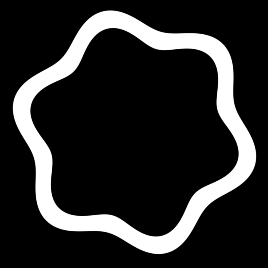
By changing the coefficient in front of the sine function and multiplying the angle by different values, one can achieve quite interesting effects.
But the main point is that now we have learned to change the radius depending on the angle. In other words, we can now draw not only perfect rings but also manipulate the shape of the ring. For example, I once really liked the effect where the ring was slightly deformed and in some places seemed to fray at the edges, then come back together. Let's create this effect, and you'll see for yourself how simple it is.
First, let's create a new method and call it DeformedCircle. It will do roughly what we've been doing in the main method: creating a ring based on the SDF for a circle and deforming its radius depending on the angle. We just need to tweak the coefficients so that the ring is deformed very slightly and the angle changes over time. I also added a variable for the angle offset in this method; this is necessary to ensure that different rings are deformed with a slight offset. This way, when overlaid, we will get small zones with the colors of the individual rings, while the main image will be white.
float DeformedCircle(float2 uv, float r, float offset) { } |
Now let's add three such circles, each with a small offset and slightly different values for the radius to make the effect more noticeable. After this, we can use the sum of all three circles as the alpha channel; the areas where there are no circles will equal zero, which will make our shader transparent. We will multiply each circle by the necessary color; I chose red, green, and blue, but I recommend experimenting with different colors. So, our main method looks something like this:
vec4 main(float2 fragCoord) { |
And the composable method code for using this shader looks like this (I'll say right away, there's nothing new in it, but just so you don't have to flip back through the book, I'll include it in full):
@Composable
fun ShadedBox() {
val shader = remember { RuntimeShader(runtimeShader) }
val time by provideTimeAsState()
Box(modifier = Modifier
.size(200.dp)
.onSizeChanged { size ->
shader.setFloatUniform(
"resolution",
size.width.toFloat(),
size.height.toFloat()
)
}
.graphicsLayer {
shader.setFloatUniform("time", time)
this.renderEffect = RenderEffect
.createRuntimeShaderEffect(
shader, "image"
)
.asComposeRenderEffect()
}
.background(Color.Black)
)
}
In the call to ShadedBox in the parent box, I added a gradient and the fake text 'loading' to make the example look more lively and beautiful. Here is the final result (if you run this on your machine, you will see that the shader is animated; it looks much more interesting in motion):
Box(modifier = Modifier .fillMaxSize() .background( brush = Brush.linearGradient( colors = listOf( Color(0xFF1F1F1F), Color(0xFF161616) ) ) ), contentAlignment = androidx.compose.ui.Alignment.Center ) { ShadedBox() Text(text = "Loading...", color = Color.White, modifier = Modifier.padding(16.dp)) } | |
Composable Code | Result |
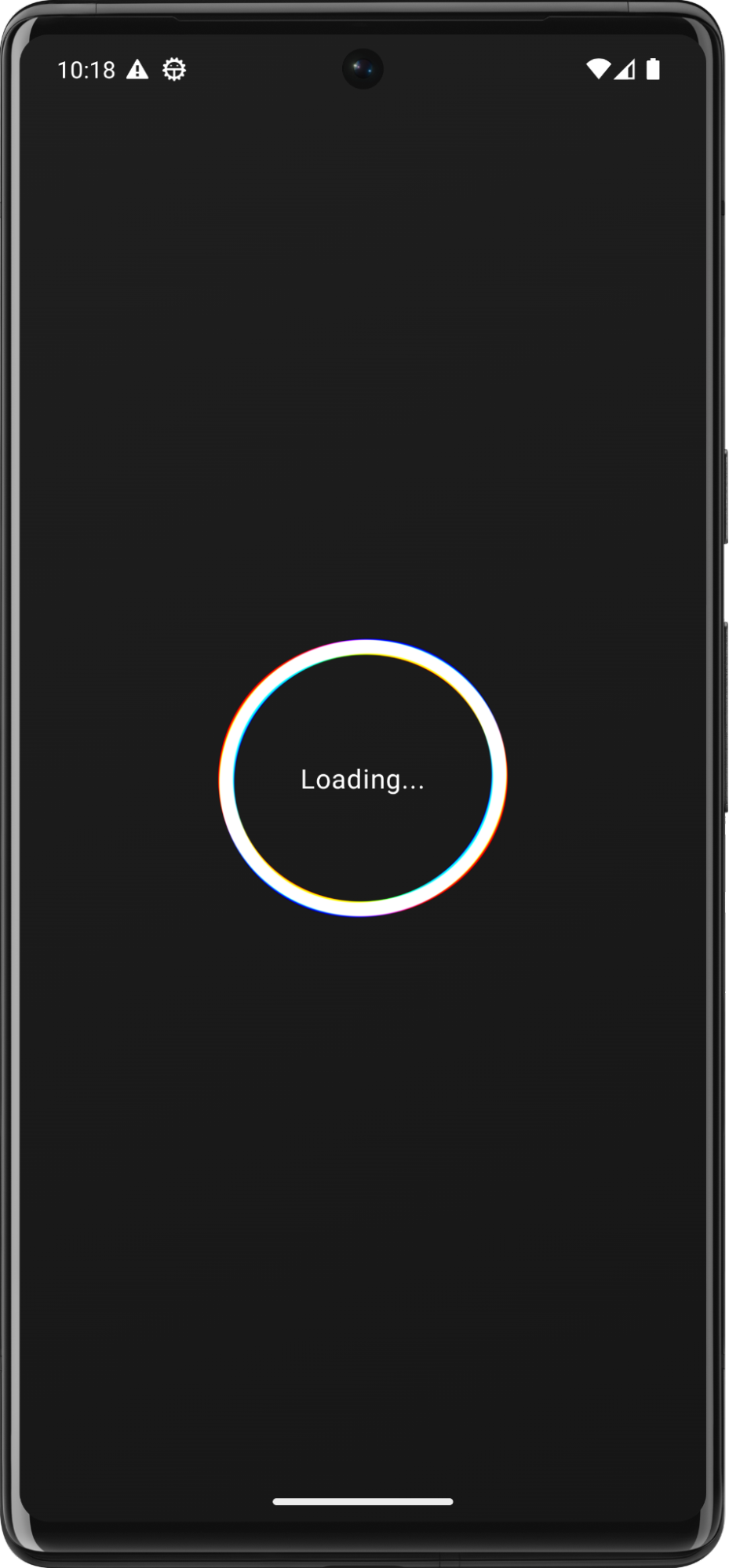
All the colors in this example are chosen to display beautifully on a dark background. I highly recommend that you pause here and practice on your own. Try passing colors depending on the current system theme, experiment with the coefficients. It might be a good idea to add more rings? In general, use your imagination to the fullest. Once you feel comfortable with this code and understand every aspect of it, come back—there's a lot of interesting stuff ahead. |
Section 06: Combining angle and smoothstep
We have already used the smoothStep method many times, which allows us to interpolate between zero and one depending on the value of a variable. But I would like to focus on this method once again. In shaders, it is quite common to need to 'enhance' or 'diminish' the effect of a function depending on certain parameters. Take a look at the sine wave graph again (I slightly changed the coefficients to make the sine wave more frequent):
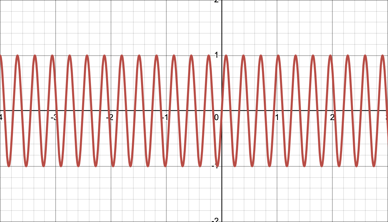
f=sin(20x)
We can already apply this to the circle's line and get a wavy curve along the perimeter. However, what if we want only part of the circle to be wavy while the rest remains straight? On the graph, this might look as follows:
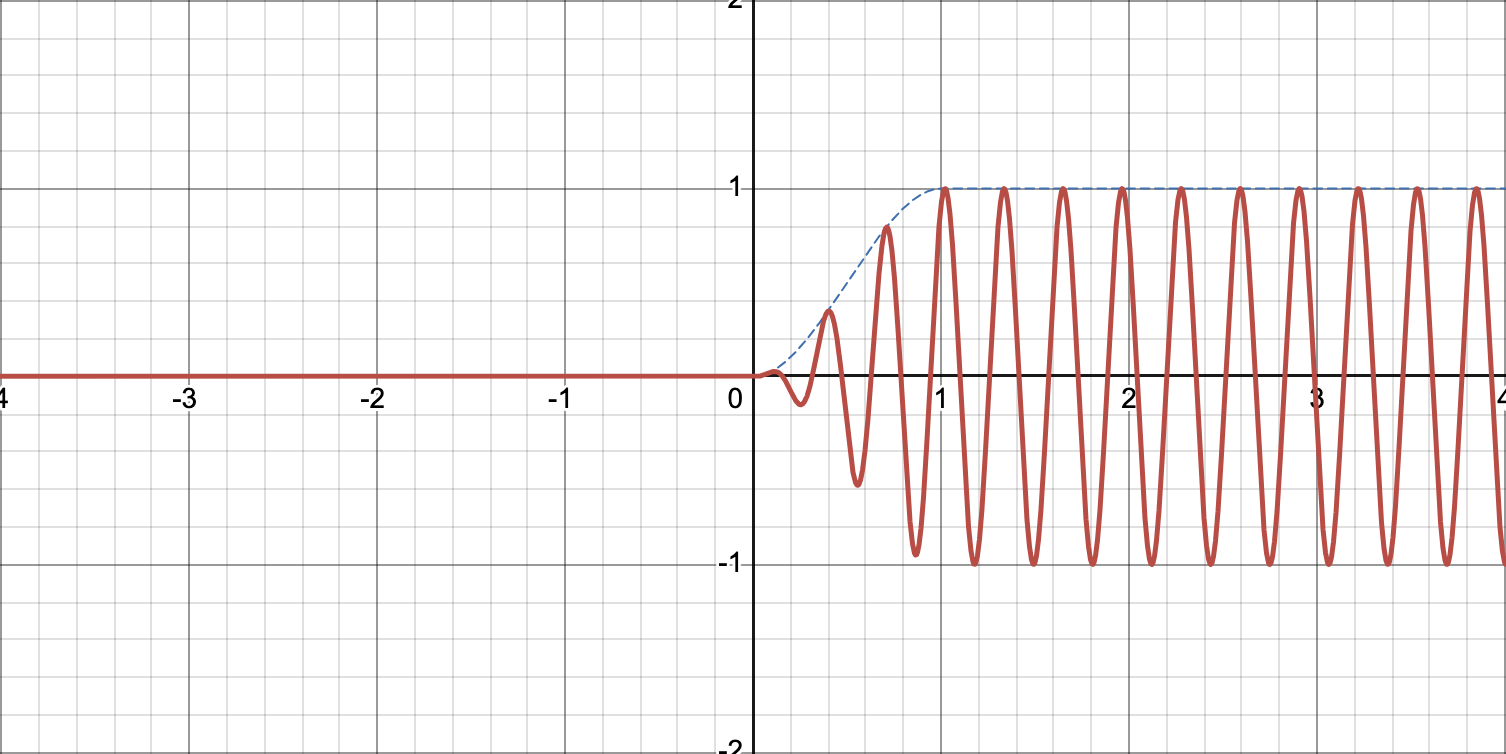
smoothstep(0,1,sin(20x))
Now this technique seems obvious, but I would like to emphasize its power. We can control the intensity of a chosen function, turning it on or off depending on the conditions we need. If we apply this technique to a circle, we can achieve, for example, the following effect
float DeformedCircle(float2 uv, float r, float offset) { float normalizedAngle = fract(angle/6.2831853 + 0.5 + reverseTime); // fract((0 .. 1) + time) * smoothstep(width, width*0.5, normalizedAngle); | |
Composable Code | Result |
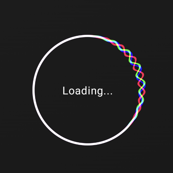
Let's take a closer look at what is happening in this shader. The first line is needed for animation, which, unfortunately, cannot be conveyed in a static format in the book. Essentially, I am slightly slowing down time and changing its sign so that the rotation goes clockwise
Then I normalized the angle. Initially, the angle changes from -π/2 to π/2, which is convenient for trigonometric functions, but if we want to interpolate some values, it's always easier to have normalized values. I divided the angle value by 2π (6.28...), thus obtaining a value in the range from -0.5 to 0.5. Then, by adding 0.5, I got a normalized value. After that, I simply added time for the animation.
float normalizedAngle = fract(angle/6.2831853 + 0.5 + reverseTime); |
It is important to note that at the end, I take the fractional part of the resulting number. This is where normalization helps us. If we simply add time to the angle value, we will quickly exceed 1 and lose the normalized values. Using fract() allows us to loop the normalizedAngle. As soon as it becomes, say, 1.1, after fract(), it will be 0.1, thus starting a second round. This allows us to create an infinite animation around the entire circle.
Next, the two lines remained unchanged compared to the previous shader. This is simply obtaining the circle and adding the sine wave as the shape of the ring. The only thing I did was change the coefficients, making the sine wave a bit more frequent and increasing the amplitude. Overall, this is a matter of personal preference, and these parameters do not affect the shader's logic itself.
float d = sdCircle(uv, r); |
Then, I set the width of the area on the circle where our function will be displayed. It makes sense to use values from 0.0 to 1.0 because we will later compare this with normalizedAngle, which changes within this range. I chose 0.4, which is slightly less than half of the circle.
The next line is the most important one in this shader. It's the reason we are doing all of this. We will apply smoothstep first from zero to the midpoint of the specified width, and then from the midpoint to the end (width), swapping the variables. By comparing these values with the normalized angle, which ranges from 0.0 to 1.0, we achieve the following: The first smoothstep method will return zero for all angles up to zero and one everywhere after half the width. The second smoothStep method will return one everywhere the angle value is less than half the width, and zero everywhere the value is greater than the width (thanks to swapping the parameters in smoothstep). In total, by multiplying these two values, we get a smooth transition of the strength value from 0 to 1 for the normalizedAngle from zero to the midpoint of our chosen width, and then a decrease from 1 to 0 up to the end of the width. In all other points, the strength variable will be equal to 0!
float strength = smoothstep(0.0, 0.5*width, normalizedAngle) |
After this, we only need to multiply our circle function by this 'strength'. Where it is zero, it will turn the entire function to zero, and where it is one, the function will return its original value. In the intermediate values, there will be a smooth transition from one state to another. That's all the magic.
float ring = d + waveFun * strength;