10 / Transform the space

Put the axes
into a matrix.

Store two familiar vectors in one value. Read the columns as transformed axes, then use them to predict what the matrix does.

25–35 min with experimentsGLSL ES 3.00 / WebGL 2After chapter 09

What we want to make

The same grid. A shorter instruction.

Compare both formulas ↓

The grid from the previous chapter already uses a matrix operation, written out as two scaled vectors. We will package those vectors into a mat2. The picture should stay the same when we switch between the two forms.

The first column of M is (0.7,0.1), and its second column is (0.2,0.6). For local=(0.6,0.5), both M times local and the expanded column sum give world=(0.52,0.36). — Two columns → two axis images → one transformationM × (0.6, 0.5) = 0.6 × M[0] + 0.5 × M[1] = (0.52, 0.36)

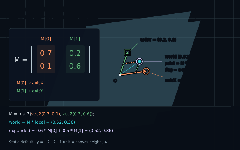
In chapter 09, we chose two axes and reconstructed a world point from local coordinates. Keep that geometry in mind. A matrix will give us a compact way to store the same choices and apply the same calculation.

Pack the axes into columns

Start with the previous chapter's axes. A GLSL mat2 stores two columns, each containing two numbers:

vec2 axisX = vec2(0.7, 0.1);
vec2 axisY = vec2(0.2, 0.6);
mat2 M = mat2(axisX, axisY);

The first vector becomes the first column. The second becomes the second column. If we print the matrix in the usual rectangular arrangement, it looks like this:

    first column   second column
        0.7             0.2
        0.1             0.6

Notice the difference between reading this picture across a row and supplying the constructor arguments. The constructor consumes a whole column before moving to the next. These two forms create the same matrix:

mat2 M = mat2(vec2(0.7, 0.1), vec2(0.2, 0.6));
// Equivalently, when supplying four scalars:
mat2 M = mat2(0.7, 0.1, 0.2, 0.6);

Choose one declaration in actual code. The two lines above show alternatives. Thinking in columns is useful because each column still has a geometric job: it tells us where one local axis step goes.

Open up the multiplication

We use column vectors in this book, with the matrix on the left:

vec2 local = vec2(0.6, 0.5);
vec2 world = M * local; // (0.52, 0.36)

This operation scales the first column by local.x, scales the second by local.y, and adds the two. GLSL indexes matrix columns starting at zero:

vec2 firstColumn = M[0];  // (0.7, 0.1)
vec2 secondColumn = M[1]; // (0.2, 0.6)
vec2 expanded = local.x * M[0] + local.y * M[1];

Nothing new happened to the point. We changed the notation for the calculation we already understand. Open it one step further to see the individual output components:

world.x = M[0].x * local.x + M[1].x * local.y;
world.y = M[0].y * local.x + M[1].y * local.y;
// world.x = 0.7 * 0.6 + 0.2 * 0.5 = 0.52
// world.y = 0.1 * 0.6 + 0.6 * 0.5 = 0.36

Each output uses one row of the printed matrix. That does not change how the matrix is constructed or indexed. In M[column][row], the first index selects the column.

Writing local * M is also legal GLSL, but it treats the vector on the left as a row vector. It is a different operation and does not follow our chosen convention. Keep M * local for the forward mapping throughout these chapters.

Read a matrix from two arrows

Apply the matrix to the three test inputs from the previous chapter:

M * vec2(1.0, 0.0) // M[0]
M * vec2(0.0, 1.0) // M[1]
M * vec2(1.0, 1.0) // M[0] + M[1]

This gives a direct way to design a transformation. Decide where one X step should land and put that destination in the first column. Decide where one Y step should land and put it in the second.

For example, send X to (1,0.5) and Y to (-0.2,1):

mat2 M = mat2(vec2(1.0, 0.5), vec2(-0.2, 1.0));
// Four-scalar form: mat2(1.0, 0.5, -0.2, 1.0)

The sum input lands at (0.8,1.5). For local=(0.6,0.5), the result is (0.5,0.8). We can obtain both predictions by adding scaled arrows, without memorizing a special formula for this tilted grid.

Identity and the origin

To leave every vector unchanged, choose the ordinary X and Y steps. This is the identity matrix:

mat2 identity = mat2(1.0, 0.0, 0.0, 1.0);
// GLSL also provides a single-scalar diagonal constructor:
mat2 sameIdentity = mat2(1.0);

A single scalar fills the diagonal and sets the remaining entries to zero. It does not fill every entry with that scalar. Identity returns local unchanged; mat2(0.0) sends every input to zero.

Every mat2, not just identity, sends the origin to itself. Multiplying both columns by zero leaves nothing to add. This also explains why a mat2 alone cannot translate all points by a nonzero offset: a translation would move the origin.

We can add an offset separately, and later we will learn how larger matrices package it. For now, keep the origin fixed. Rotation, scaling, shearing, reflection, and collapse can all fit this rule.

What linear means here

A matrix multiplication preserves addition and scalar multiplication:

M * (a + b) = M * a + M * b
M * (s * a) = s * (M * a)

These are mathematical equalities, not GLSL assignments. To see the first one, expand the column sum. The coefficient of M[0] is a.x + b.x; distributing that multiplication gives the two X contributions. The same happens for the Y column. Group the parts for a and b, and we have the right-hand side.

Scaling a vector scales both of its coordinates, so it scales both column contributions by the same amount. Together these properties make the mapping linear. The parallelogram formed by a and b maps to the parallelogram formed by their images, though it can flatten to a line or point.

Using the exercise matrix, let a=(0.2,0.1) and b=(0.1,0.3). Their images are (0.18,0.2) and (0.04,0.35). Adding gives (0.22,0.55), the same result as transforming a+b=(0.3,0.4). Doubling a gives (0.36,0.4) after transformation.

These identities hold in exact arithmetic. Shader calculations may round their last digits differently, especially after cancellation. Compare with a small tolerance rather than expecting every alternative expression to produce identical bits.

Dependent columns are allowed in a matrix. They no longer provide a full two-dimensional basis, but the forward product remains defined and linear. No inverse is needed to draw such a collapsed result.

Catch a row-column mistake

The exercise matrix prints as two rows: (1,-0.2) and (0.5,1). Pasting those rows directly into a four-scalar constructor creates the wrong columns:

mat2 wrong = mat2(1.0, -0.2, 0.5, 1.0);
// Wrong column 0: (1.0, -0.2)
// Wrong column 1: (0.5, 1.0)

This exchanges rows and columns, called a transpose. The code compiles, so the compiler cannot diagnose our geometric intention. The unit test inputs can: X now goes to (1,-0.2), and Y goes to (0.5,1). Our local (0.6,0.5) lands at (0.85,0.38) instead of (0.5,0.8).

Writing the constructor as two explicit vec2 columns makes this mistake easier to spot. In the lab, each column has the same color as its corresponding axis arrow.

Try it

Read the columns. Predict the point.

LIVE GLSL / WEBGL 2

Edit the four entries or drag the axis handles. Switch Matrix and Expanded: the point and grid should stay in the same places. A comparison ring marks the result of the other expression on the GPU.

The fixed view spans −2 to 2 world units vertically, so the exercise's unit parallelogram fits on screen. Both axes use the same scale: one world unit occupies a quarter of the canvas height.

Static default matrix: its columns are (0.7,0.1) and (0.2,0.6). Matrix multiplication and the expanded column sum both send local=(0.6,0.5) to world=(0.52,0.36). A pale comparison ring surrounds the cyan result point.

Orange circle: M[0] · axis XGreen square: M[1] · axis YCyan point: selected expressionPale ring: other GPU expression

Fixed view half-height: 2. Equal coordinate units; y runs from −2 to 2. One unit is one quarter of the canvas height.

Matrix mode: the cyan point and mapped grid use M * local. The pale ring uses the expanded column sum. Their positions should agree.

Small solid orange and green markers show the weighted column parts; dashed copies complete their parallelogram. The mapped grid is a finite patch, −2 to 2 on both local axes, every 0.5. Each segment endpoint uses the selected forward expression.

Two columns, four numbers

Expression

M[0].x

M[1].x

M[0].y

M[1].y

Rows read across; each colored column is one full axis. Entries range from −1 to 1. The constructor takes the entire orange column first, then the green column.

mat2(vec2(0.7, 0.1), vec2(0.2, 0.6))

Matrix presets keep local components. Transpose entries swaps the two off-diagonal values: M[0].y and M[1].x. This changes which numbers form each column.

Move handle

Local input vector

local.x

local.y

Local presets keep the matrix. Local components range from −2 to 2.

Show original grid Show local grid

Reset lab restores the previous-basis matrix, local=(0.6,0.5), Matrix mode, and both grids. Reset code restores the shader. Reset identity changes only the matrix entries.

Preparing the live shader.

M[0] · first column · M × (1,0): (0.70000, 0.10000)
M[1] · second column · M × (0,1): (0.20000, 0.60000)
Local input vector: (0.60000, 0.50000)
Zero stays zero · M × (0,0): (0.00000, 0.00000)
Matrix result · M * local: (0.52000, 0.36000)
Expanded result · weighted columns: (0.52000, 0.36000)
Host comparison · max component difference: 0.00e+0
Selected world point: (0.52000, 0.36000)

These columns point in two independent directions. Their full lengths remain part of the multiplication.

The world point is inside the fixed view.

The numbers are host float32 reference calculations for the built-in formulas, not GPU measurements. Both host calculations use explicitly rounded products and sums, so their difference is normally zero. The GPU may round the last digits differently. In the live preview, the point and comparison ring show the two expressions evaluated on the GPU; shader edits affect those drawings but do not change the readouts or constructor display. Column diagnostics use a relative near-parallel tolerance of 0.000001 and never change the entries.

Drag the orange circular or green square column handle. Clicking near a handle selects it; clicking elsewhere places the selected endpoint there, within the entry limits. The Move handle menu chooses the column explicitly. Focus the diagram and use arrow keys to move its endpoint by 0.05 world units, or Shift for 0.25. On touch screens, tap or use the controls; a swipe scrolls the page.

Open the complete shader edit · run · reset

The host supplies uAxisX, uAxisY, uLocal, uMode (0 for Matrix, 1 for Expanded), the two grid toggles, and uResolution. The constructor packs columns, and the selected expression maps both the point and the finite grid. All drawing helpers are supplied here.

#version 300 es
precision highp float;

uniform vec2 uResolution;
uniform vec2 uAxisX; // The full axis vectors: their lengths matter.
uniform vec2 uAxisY;
uniform vec2 uLocal;
uniform int uMode; // 0: matrix multiplication; 1: expanded column sum.
uniform int uShowOriginalGrid;
uniform int uShowLocalGrid;
out vec4 fragColor;

// Supplied drawing helpers. They handle a segment with coincident endpoints.
float segmentDistance(vec2 p, vec2 a, vec2 b) {
    vec2 ab = b - a;
    float lenSq = dot(ab, ab);
    if (lenSq <= 0.00000001) return length(p - a);
    float t = clamp(dot(p - a, ab) / lenSq, 0.0, 1.0);
    return length(p - (a + t * ab));
}

float stroke(float distanceToLine, float halfWidth, float pixelSize) {
    return 1.0 - smoothstep(halfWidth, halfWidth + pixelSize, distanceToLine);
}

float arrow(vec2 p, vec2 a, vec2 b, float halfWidth, float pixelSize) {
    vec2 delta = b - a;
    float len = length(delta);
    if (len <= 0.0001) return 0.0;
    vec2 direction = delta / len;
    vec2 side = vec2(-direction.y, direction.x);
    float head = min(0.10, len * 0.35);
    vec2 left = b - direction * head + side * head * 0.5;
    vec2 right = b - direction * head - side * head * 0.5;
    float d = min(segmentDistance(p, a, b),
        min(segmentDistance(p, b, left), segmentDistance(p, b, right)));
    return stroke(d, halfWidth, pixelSize);
}

float dashedSegment(vec2 p, vec2 a, vec2 b, float halfWidth, float pixelSize) {
    float dash = step(0.04, mod(length(p - a), 0.08));
    return stroke(segmentDistance(p, a, b), halfWidth, pixelSize) * dash;
}

// Every grid endpoint uses the selected forward expression too.
vec2 toWorld(vec2 local) {
    mat2 M = mat2(uAxisX, uAxisY); // Constructor arguments are columns.
    if (uMode == 0) return M * local;
    return local.x * M[0] + local.y * M[1];
}

void main() {
    // A fixed view: half-height 2; one unit is one quarter of the buffer height.
    vec2 p = 2.0 * (2.0 * gl_FragCoord.xy - uResolution) / uResolution.y;
    float pixelSize = 4.0 / uResolution.y;

// The lesson: the constructor packs the two full axes as columns.
    mat2 M = mat2(uAxisX, uAxisY);
    vec2 local = uLocal;
    vec2 world = M * local;
    vec2 expanded = local.x * M[0] + local.y * M[1];
    vec2 comparison = expanded;
    if (uMode == 1) {
        comparison = world;
        world = expanded;
    }
    vec2 axisX = M[0];
    vec2 axisY = M[1];
    vec2 firstPart = local.x * M[0];
    vec2 secondPart = local.y * M[1];

vec3 color = vec3(0.035, 0.055, 0.08);
    vec3 outline = vec3(0.015, 0.025, 0.04);
    vec3 xColor = vec3(1.0, 0.57, 0.28);
    vec3 yColor = vec3(0.40, 0.87, 0.56);
    vec3 pointColor = vec3(0.24, 0.88, 0.94);
    vec3 comparisonColor = vec3(0.93, 0.85, 1.0);
    vec2 origin = vec2(0.0);

if (uShowOriginalGrid == 1) {
        vec2 gridDistance = abs(mod(p + 0.25, 0.5) - 0.25);
        color = mix(color, vec3(0.35, 0.42, 0.47),
            stroke(min(gridDistance.x, gridDistance.y), 0.0, pixelSize) * 0.4);
        color = mix(color, xColor, stroke(abs(p.y), 0.0, pixelSize) * 0.25);
        color = mix(color, yColor, stroke(abs(p.x), 0.0, pixelSize) * 0.25);
    }

// A finite local patch: [-2,2] on both axes, with a line every 0.5.
    // Each pair of endpoints is mapped forward. No inverse is needed.
    if (uShowLocalGrid == 1) {
        float alongX = 100.0;
        float alongY = 100.0;
        for (int i = -4; i <= 4; i++) {
            float coordinate = float(i) * 0.5;
            alongX = min(alongX, segmentDistance(p,
                toWorld(vec2(-2.0, coordinate)), toWorld(vec2(2.0, coordinate))));
            alongY = min(alongY, segmentDistance(p,
                toWorld(vec2(coordinate, -2.0)), toWorld(vec2(coordinate, 2.0))));
        }
        color = mix(color, xColor, stroke(alongX, pixelSize * 0.3, pixelSize) * 0.27);
        color = mix(color, yColor, stroke(alongY, pixelSize * 0.3, pixelSize) * 0.27);
    }

// Parallelogram: the dashed sides are translated copies of the parts.
    float translated = max(
        dashedSegment(p, firstPart, world, pixelSize * 2.5, pixelSize),
        dashedSegment(p, secondPart, world, pixelSize * 2.5, pixelSize));
    color = mix(color, outline, translated);
    color = mix(color, yColor, dashedSegment(p, firstPart, world, pixelSize, pixelSize));
    color = mix(color, xColor, dashedSegment(p, secondPart, world, pixelSize, pixelSize));
    color = mix(color, outline, arrow(p, origin, world, pixelSize * 2.5, pixelSize));
    color = mix(color, pointColor, arrow(p, origin, world, pixelSize * 0.5, pixelSize));

// Full axes have hollow handles: X is a circle, Y is a square.
    color = mix(color, outline, arrow(p, origin, axisX, pixelSize * 2.8, pixelSize));
    color = mix(color, xColor, arrow(p, origin, axisX, pixelSize, pixelSize));
    color = mix(color, outline, arrow(p, origin, axisY, pixelSize * 2.8, pixelSize));
    color = mix(color, yColor, arrow(p, origin, axisY, pixelSize, pixelSize));
    color = mix(color, xColor, stroke(segmentDistance(p, origin, firstPart), pixelSize * 1.5, pixelSize));
    color = mix(color, yColor, stroke(segmentDistance(p, origin, secondPart), pixelSize * 1.5, pixelSize));
    float xHandle = abs(length(p - axisX) - 0.06);
    vec2 fromY = abs(p - axisY);
    float yHandle = abs(max(fromY.x, fromY.y) - 0.05);
    color = mix(color, outline, stroke(min(xHandle, yHandle), pixelSize * 2.5, pixelSize));
    color = mix(color, xColor, stroke(xHandle, pixelSize, pixelSize));
    color = mix(color, yColor, stroke(yHandle, pixelSize, pixelSize));

// Small solid part markers are distinct from the hollow axis handles.
    color = mix(color, outline, 1.0 - smoothstep(0.036, 0.036 + pixelSize, length(p - firstPart)));
    color = mix(color, xColor, 1.0 - smoothstep(0.023, 0.023 + pixelSize, length(p - firstPart)));
    color = mix(color, outline, 1.0 - smoothstep(0.036, 0.036 + pixelSize, length(p - secondPart)));
    color = mix(color, yColor, 1.0 - smoothstep(0.023, 0.023 + pixelSize, length(p - secondPart)));
    color = mix(color, outline, 1.0 - smoothstep(0.055, 0.055 + pixelSize, length(p - world)));
    color = mix(color, pointColor, 1.0 - smoothstep(0.035, 0.035 + pixelSize, length(p - world)));
    // The ring uses the other expression evaluated by this shader on the GPU.
    float comparisonRing = abs(length(p - comparison) - 0.085);
    color = mix(color, outline, stroke(comparisonRing, pixelSize * 2.5, pixelSize));
    color = mix(color, comparisonColor, stroke(comparisonRing, pixelSize, pixelSize));
    color = mix(color, vec3(0.95), 1.0 - smoothstep(0.012, 0.012 + pixelSize, length(p)));
    fragColor = vec4(color, 1.0);
}

⌘ / Ctrl + Enter to run

Both modes map the finite local grid forward, from coordinates −2 to 2 in steps of 0.5. There is no inverse sampling in this example. The host code supplies entries and local coordinates; numerical references stay tied to the built-in formulas when the shader is edited.

A complete matrix comparison shader

Paste this smaller version into the editor. It draws the columns, a point from the selected method, and a ring from the other method. The longer default shader supplies the grid and contribution guides.

#version 300 es
precision highp float;
uniform vec2 uResolution;
uniform vec2 uAxisX;
uniform vec2 uAxisY;
uniform vec2 uLocal;
uniform int uMode; // 0 = Matrix, 1 = Expanded.
out vec4 fragColor;

float segmentDistance(vec2 p, vec2 a, vec2 b) {
    vec2 ab = b - a;
    float lenSq = dot(ab, ab);
    float t = lenSq > 0.00000001
        ? clamp(dot(p - a, ab) / lenSq, 0.0, 1.0) : 0.0;
    return length(p - (a + t * ab));
}

float stroke(float d, float width, float edge) {
    return 1.0 - smoothstep(width, width + edge, d);
}

void main() {
    // Fixed view half-height: 2 world units.
    vec2 p = 2.0 * (2.0 * gl_FragCoord.xy - uResolution) / uResolution.y;
    float edge = 4.0 / uResolution.y;
    mat2 M = mat2(uAxisX, uAxisY);
    vec2 world = M * uLocal;
    vec2 expanded = uLocal.x * M[0] + uLocal.y * M[1];
    vec2 shown = uMode == 0 ? world : expanded;
    vec2 other = uMode == 0 ? expanded : world;
    vec3 color = vec3(0.04, 0.06, 0.09);
    color = mix(color, vec3(1.0, 0.57, 0.28),
        stroke(segmentDistance(p, vec2(0.0), M[0]), 0.012, edge));
    color = mix(color, vec3(0.40, 0.87, 0.56),
        stroke(segmentDistance(p, vec2(0.0), M[1]), 0.012, edge));
    color = mix(color, vec3(0.24, 0.88, 0.94),
        1.0 - smoothstep(0.035, 0.035 + edge, length(p - shown)));
    float comparisonRing = abs(length(p - other) - 0.065);
    color = mix(color, vec3(0.92, 0.86, 1.0),
        stroke(comparisonRing, 0.008, edge));
    fragColor = vec4(color, 1.0);
}

The drawing uses world-space distances and a fixed view scale. Those choices make the diagram readable; they are not part of matrix multiplication. If an edited expression disagrees with the other one, the point can leave the comparison ring.

Your turn

Use Reset lab and Reset code first.

Construct a matrix that sends X to (1,0.5) and Y to (-0.2,1). Enter the four numbers, or use Exercise axes to check your work. Predict the results for local (1,0), (0,1), and (1,1).
Set local=(0.6,0.5). Switch Matrix and Expanded and compare the point with its ring. Then choose Transpose entries. Predict the new columns and world point before checking.
Restore Exercise axes. Test the linearity example: compare the results for a=(0.2,0.1), b=(0.1,0.3), and a+b=(0.3,0.4). Add the first two results yourself. Then try local=(0.4,0.2), twice a.
Use Reset identity and check that the output equals the input. Test local (0,0) with several matrices. Finally try Zero matrix and Collinear: explain why multiplication still works but a full plane is no longer preserved.

A hint

Write the constructor as two vec2 columns before placing the entries into the rectangular display. The first unit test reads the first column; the second reads the second column. Matrix and Expanded cannot tell whether you chose the intended matrix: they can agree on a wrong one.

Check your result

The correct constructor is mat2(1.0,0.5,-0.2,1.0). The three test results are (1,0.5), (-0.2,1), and (0.8,1.5). Local (0.6,0.5) gives (0.5,0.8). After transposition, the columns are (1,-0.2) and (0.5,1), and the same local input gives (0.85,0.38). Both methods still agree for that different matrix.

The linearity results are (0.18,0.2), (0.04,0.35), and their sum (0.22,0.55). Twice a gives (0.36,0.4). Identity changes nothing; every matrix preserves the zero input. Zero matrix collapses the whole plane to the origin, while the Collinear preset maps it to a line.

What you can do now

Build a matrix from two desired axis images and verify it with (1,0), (0,1), and (1,1). Explain why its product matches the expanded column sum and why it cannot translate the origin. Next, we will choose columns that rotate the plane.