We can now compose transforms, reverse them, and recognize collapse. This chapter puts those skills into a small transform editor. The new piece is a matrix that includes translation instead of keeping it beside the matrix.
Give translation a column
A linear mat2 cannot move the origin. Multiplying any matrix by the zero vector still gives zero. Our previous rule therefore needed an extra term:
vec2 world = A * local + offset;A linear transformation followed by a translation is an affine transformation. For the invertible transforms used here, straight lines remain straight and parallel lines remain parallel. A singular affine map can collapse a line to a point. When offset is nonzero, it is not a linear map of the original 2D plane, because it no longer fixes the origin.
Add one component to the input. For a point, set this extra component to 1. It gives a third matrix column something to multiply:
mat3 M = mat3(vec3(A[0], 0.0),
              vec3(A[1], 0.0),
              vec3(offset, 1.0));
vec3 world = M * vec3(local, 1.0);
The constructor still takes columns. The first two contain the linear axes, extended with zero. The third contains the offset, extended with one. Displayed in rows, the same matrix is:
[ A[0].x   A[1].x   offset.x ]
[ A[0].y   A[1].y   offset.y ]
[    0        0        1     ]
Multiplication adds local.x times the first column, local.y times the second, and 1 times the third. The first two output components are exactly A*local+offset. The last component remains 1.
These are homogeneous coordinates. We call the extra component w, although it occupies .z in this GLSL vec3. It is not a new depth coordinate in this chapter. Our affine matrices keep the bottom row (0,0,1), so points keep w=1 and taking .xy gives their ordinary 2D coordinates. Perspective will need a separate step later.
Choose point or direction
A point has a position. A direction is a displacement between positions. Moving the entire drawing should move its points without adding that movement to each displacement.
vec2 worldPoint = (M * vec3(localPoint, 1.0)).xy;
vec2 worldDirection = (M * vec3(localDirection, 0.0)).xy;
With w=0, the third column contributes zero. Rotation and scale still act on the direction; translation does not. A direction is not automatically a unit vector, and non-uniform scale can change both its length and its angle.
For translation alone by (0.6,−0.3), the input (0.4,0.2) becomes point (1,−0.1), but direction (0.4,0.2). The lab draws the direction arrow from the fixed world origin so you can see that its components stay unchanged as translation moves the card.
This convention also follows from subtracting points. If two points become A*p+offset and A*q+offset, their difference is A*(p−q): the offsets cancel. Their homogeneous components subtract to 1−1=0. That is why a displacement belongs in the w=0 form.
Build the whole chain
Make a translation helper by using identity axes and placing the offset in the third column:
mat3 translation(vec2 t) {
    return mat3(vec3(1.0, 0.0, 0.0),
                vec3(0.0, 1.0, 0.0),
                vec3(t, 1.0));
}
Extend rotation and scale in the same way, but give them a third column (0,0,1). The complete shader below includes both constructors. Now their composition is ordinary matrix multiplication:
mat3 M = translation(offset) * rotation(angle) * scaling(scale);Read from the input outward: scale first, rotate second, translate last. The resulting matrix stores the complete mapping. Reordering the factors changes the result, just as in chapter 13.
For two affine maps A₂*(A₁*p+t₁)+t₂, the combined linear part is A₂*A₁ and the combined offset is A₂*t₁+t₂. Multiplying their mat3 matrices carries out this bookkeeping for us. Earlier translations may be rotated or scaled by later factors.
Put the pivot in the product
Let c be the pivot in the card's original coordinate system. It may be inside or outside the card. To scale and rotate around it, first subtract c, apply scale and rotation, then add c back:
mat3 aroundPivot = translation(c) * rotation(angle)
                 * scaling(scale) * translation(-c);
mat3 M = translation(offset) * aroundPivot;
Before the final offset, the pivot stays fixed: c becomes zero, the linear operations keep it zero, and adding c restores it. After the offset, its world position is c+offset. Changing the pivot does not mean moving the world origin.
Writing A=R*S, the complete rule expands to A*(local−c)+c+offset. The third column therefore contains the effective translation b=c+offset−A*c, not simply the offset control. The first two columns still contain A.
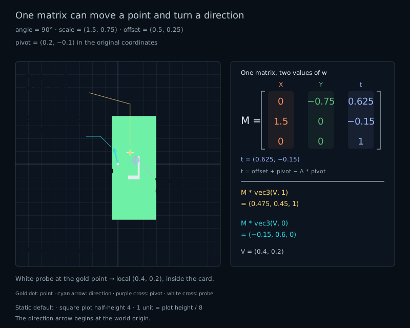
At Combined, angle=90°, scale=(1.5,0.75), c=(0.2,−0.1), and offset=(0.5,0.25). The local sample V=(0.4,0.2) passes through (0.2,0.3), (0.3,0.225), (−0.225,0.3), (−0.025,0.2), then world=(0.475,0.45).
// Combined, ideal values shown in row order:
[ 0    -0.75    0.625 ]
[ 1.5   0      -0.15  ]
[ 0     0       1     ]
As a direction, the same input becomes (−0.15,0.6). Every translation factor multiplies w=0, including the pivot translations. Changing offset or pivot leaves that direction unchanged while the card and point may move.
Test the pointer locally
Our card is a rectangle with local half-size (0.6,0.4). A rotated rectangle is awkward to test in world coordinates. Its local test stays short:
vec2 localPointer = (inverse(M) * vec3(pointerWorld, 1.0)).xy;
bool inside = all(lessThanEqual(abs(localPointer), vec2(0.6, 0.4)));
The pointer is a world point, so it needs w=1. The inverse removes the entire forward chain, including its effective translation. At Combined, world pointer (0.475,0.45) recovers local (0.4,0.2), which is inside the card.
Use the same inverse for rendering each pixel and for testing the pointer. The card's mask and interaction then share one coordinate system. The host readouts mirror the built-in formulas with float32 reference arithmetic; the shader performs its own lookup and highlight. Editing the shader does not update those references.
The hit test includes the mathematical rectangle boundary. Float rounding near that boundary can change the result, and the antialiased visual edge can extend outside it. Test clearly inside or outside when checking the transformation; do not treat a faint edge pixel as an exact hit boundary.
Scale stays in [0.5,2] on both axes, so this family has an inverse throughout. Its linear determinant lies in [0.25,4]. We avoid collapse here to keep pointer interaction available; chapter 15 explains what a rejected inverse needs instead.